Layered Meshing 03: Meshing complex geophysical domains

The new “layered meshing” interface in Salvus allows us to declaratively build meshes for complex multi-layered domains. In this example we’ll give an overview of how it can be used to create a mesh for a chunk of Monterey bay which includes topography, bathymetry, thin near-surface layers, and the ocean itself. We’ll also use this opportunity to give a refresher on the different “policy” types, and how they interact to form our final mesh. Let’s get started!

As always, the first step is to import the Salvus Python environment. Here we’ll add an extra import to the canonical Salvus namespace to bring the layered meshing API into scope.

Selecting our domain

As outlined in the 3D Surface Topography tutorial, the first thing we want to do when working with areas of Earth’s surface is to define our domain. We’ll be working in UTM coordinates, and a convenient way to handle coordinate conversions is to use the specialized UtmDomain.from_spherical_chunk constructor that takes WGS84 coordinates and converts them to an appropriate UTM domain. The UTM zone and coordinates could of course also be specified directly.

We choose a small box around Monterey, California, as below.

All looks good. We see that we’ve selected a domain that is mostly comprised of ocean, and which abuts Monterey to the east.

Downloading topography and bathymetry

As outlined in the 3D Surface Topography tutorial, we’ll use the GMRT web service to automatically download topography and bathymetry for our domain. This is simple to do via the domain object itself.

As this topography file is in spherical coordinates, we’ll need to again perform a coordinate transform to get this into the coordinates of Monterey’s UTM zone. Salvus has a built-in transformation function to do exactly this, which takes the domain’s UTM definition, and can be executed as below.

As is true for the volumetric models we’ll encounter shortly, the result of this transformation is an xarray DataArray. These datasets are simple to manipulate and visualize, and we can for instance plot the digital elevation model in the notebook by simply plotting the `xarray“ dataset.

Looks like Monterey! We can see the classic subsea channel.

Creating a layered model

Before we begin the meshing process, its a good idea to think carefully at the model we’ll want to mesh. The following setup is hypothetical, but derived from several common properties present on the exploration / monitoring scale. Let’s go over the layers we’ll be considering.

Materials

A “layer” in this context refers to a material bounded by two interfaces. We’ll start by exploring the definitions of the materials.

Layer 1: Ocean

As we’ve mentioned earlier our chosen domain straddles the shoreline, and we’ll want to model the effects of the ocean itself. So, we’ll first need to consider how to define the ocean’s properties. Let’s first define the properties and then loop back to explain the different components.

OK, let’s unpack that.

• depth = ...: The definition of depth above introduces the ability to define “analytic” parameters with respect to model coordinates. Possible values here would be one of x, y, z, v, or depth. x, y, and z are the three Cartesian dimensions of our model, while v is a generic coordinate corresponding to the vertical coordinate in a given dimension (y in 2-D and z in 3-D). depth, which we’ve used, is similar to v in that it is generic over the domain’s dimension, but is defined instead with respect to the top surface of the domain. Analytic parameters are defined using sympy symbols.

• ocean_properties = ...: Here we declare the material that defines our ocean — an acoustic material defined by P-wave velocity and density. A variety of other materials, including multiple parameterizations for many, can be found in the layered meshing [materials](https://mondaic.com/docs/references/python_api/salvus/mesh/layered_meshing/material) submodule. Each argument to the .from_params(...) method associated with a given material’s parameterization can take one of a constant value (as we’ve done for vp), a symbolic expression (as we’ve done for rho), or an xarray DataArray (described below).

Layer 2: Near-surface

Below our ocean we’ll define an elastic near-surface geotechnical layer that is characterized by vertically and laterally varying parameters. Let’s do this below, and again circle back to explain the particulars.

Let’s again unpack the above.

• rho = ...: The definition of density here introduces the use of an xarray.DataArray as a way to define discrete parameters. xarray is a fantastic toolbox for working with regularly sampled data, and a host of tutorials and examples can be found on its website. Here we define a simple density model with two values that are associated with the coordinates "v_relative". "v_relative" is a parameter that is currently exclusive to discrete, xarray-based parameter representations, and is a flag telling Salvus to interpolate the model solely within its host layer, with the value at v_relative=1.0 corresponding to the value at the layer’s top interface, and v_relative=0.0 to the value at the layer’s bottom interface. This is handy to ensure that your parameter definition shrinks and stretches with any mesh deformations, as we’ll se below. We could have alternatively used any of the other coordinate values outlined in the discussion surrounding analytic parameters, in which case the specified locations would be interpreted as absolute with respect to our coordinate system. The presence of v in the phrase v_relative holds the same meaning as before, in that it is a generalization of the vertical coordinate name.

• vs = ...: Here we expand on the definition of rho above by defining a 2-D model for vs. We again use v_relative to signal that we want the variation in the vertical direction to occur exclusively within the layer, but in this case also include an x coordinate to signal variation along the x direction. The values of the x coordinate here are absolute with respect to the UTM zone we’ll be working in. In summary, then, we’ve defined a vs model that vertically varies between 300.0 and 600.0 m/s in the east, which increases to between 600.0 and 900.0 m/s as we travel west. Note that these x values do not span the entirety of our domain but they, along with the missing y coordinate, will be extruded to fit.

• vp = ...: Here we simply create a vp model by scaling our vs model by the square root of 3, which corresponds to a material with a Poisson’s ratio of 0.25.

Layer 3: Compacted sediments

Below the near surface layer we defined a third layer which represents a collection of compacted sediments. The definition of this layer is very similar to that of the above.

The only notable differences here with respect to layer 2 is the inclusion of a constant density, and the fact that in this case our vs / vp values vary only with the vertical coordinate. As previously, the inclusion of "v_relative" informs Salvus that the materials should be interpolated with respect to the layer’s vertical bounds, and thus be shrunk or stretched accordingly.

Layer 4: Bedrock

Our final layer describes the bedrock model below the compacted sediments, and is defined below.

Here we define all three parameters as varying solely in the vertical direction, with one important change to what we’ve seen above. Similarly to how we define the density in the ocean, we use "depth" as the coordinate of interest. This now means that, rather than interpolating uniformly between the layer’s bounding interfaces, we instead interpret the coordinates as the absolute depth below the domain’s top surface.

For any discrete model specified as an xarray dataset, we have a choice to define a a model in any of the 0 to n dimensions of the domain, or any subset of them. The missing dimensions will be added accordingly, and if they defined model does not span the domain’s extent in any of these dimensions it will additionally be extruded to do so. The only restriction is that multiple values can not be specified for a single coordinate, i.e. "depth" and "v_relative" would be invalid.

Interfaces

As specified above, a “layer” is a collection of materials and bounding interfaces, and it is now time to consider the interfaces themselves. Before doing this, its helpful to consider a schematic of what we’re envisioning.

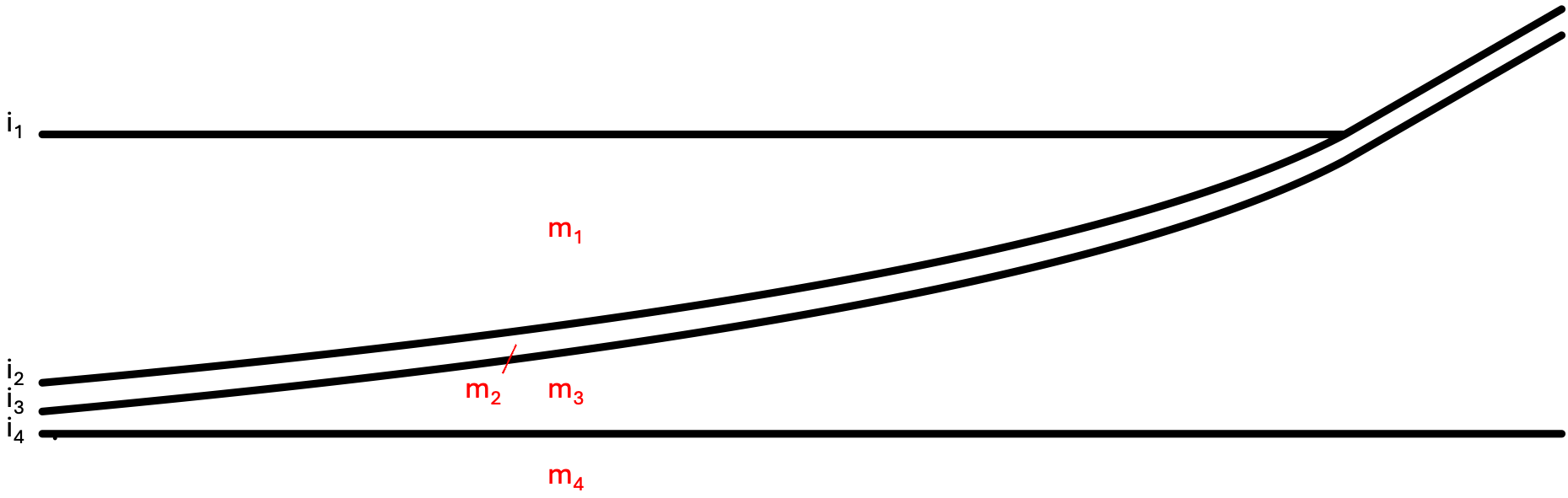
Above, we’re considering an x-z cross section, moving east along the horizontal axis. We can associate the four materials we’ve defined with $m_{n}$ in the schematic, corresponding to the ocean, near-surface, sediment, and bedrock layers respectively. If it was not already apparent that the ocean layer would not span the entire domain, we now see that this will be the case — indeed the “bathymetry” becomes “topography” as we move onshore. In general, explicit layers which with a vanishing thickness are not supported in Salvus, and their future implementation is on Mondaic’s longer term technical roadmap. A special case, however, of a vanishing top layer is currently supported, and we’ll see below how to instruct the meshing algorithms that this is our intent.

Interface 1: Ocean surface

With this basic skeleton in mind, let’s now go and create out interfaces. First, we start with the ocean surface.

Here we encounter our first type of interface: a Hyperplane. A Hyperplane is a simple interface in that it is always flat in whichever coordinate system we choose. In this case we are requesting a flat interface at an absolute elevation of 0.0 which defines our ocean surface, a Hyperplane in spherical coordinates would represent a constant radial value. The value of 0.0 used in this case is relevant in the context of our UTM domain, where elevation is provided with respect to mean sea level.

Interface 2: Topography / bathymetry

More interesting than a flat interface is the one defined by the topography file we downloaded above. Bringing this in to our layered mesh is simple. Here we are directly taking the xarray representation of our digital elevation model (DEM) from the GMRT dataset we downloaded, and specifying that it is also with reference to mean sea level.

Interface 3: Bottom of near-surface layer

When looking at our schematic above, we see that the bottom of the near-surface layer should follow the curvature of our surface topography. The simplest way to implement this is just to take our surface topography and shift it down by some amount. To do this we can use the .map(...) attribute on our newly-created surface topography object. This gives us access to the xarray representation of the interface, and allows us to assign a new reference elevation. Below, we shift the interface down by 200 meters, giving us a layer with a consistent thickness of 200 m. It is also possible to use the map interface to, for example, scale our topography or perform other operations while keeping its basic structure constant.

Interface 4: Bottom of sediment layer

The final interface we specified in our schematic was the bottom of the sediment layer. Here we again choose a Hyperplane to declare our intent that this interface is flat in our Cartesian coordinate system. We set the depth of this layer to 4km below the top of the domain. Importantly, this is below the bottom of the near-surface layer, so we do not have another layer crossing boundaries.

Interface 5: Bottom of domain

What we have not specified in our schematic, but which is of course important, is a definition of the bottom of our domain. While this can be encoded in our Domain object, the UTMDomain classification leaves the top and bottom bounds of the domain undefined and expects them to be specified at the time of mesh generation. Our top surface has already been well defined — by the ocean_surface and the topography interfaces, and it thus remains to define our bottom interface. Below we define yet another Hyperplane to specify the bottom of the domain, here at a depth of 10km below the surface.

Pulling everything into a layered model

With our materials and interfaces defined, we can now pull everything together in a single LayeredModel. This class is accessible from the layered_meshing module we’ve already imported, and simple takes a list of alternating interfaces and layers.

Generating our mesh

Everything above can now be passed to the meshing entry point: the mesh_from_domain function from the layered_meshing module. This takes our domain and our layered model which we just defined, as well as a minimal MeshResolution object that encodes properties like the order of model representation, the elements per wavelength we’re targeting, and the reference frequency for which we want to generate the mesh. Let’s go ahead and execute it with the layered model we’ve put together.

Troubleshooting

Hmm… that didn’t quite work. All is not lost, though, and the error message above gives us insight into what’s going on. Specifically, we see:

ValueError: After interpolation, layer boundaries have been found to cross.

This is, of course, not unexpected, as we discussed above that support for crossing and “pinched-out” layers is only possible in specific circumstances. As we’re pinching out only the top layer of the mesh, this application is indeed supported, and to activate this support we need to shortly discuss the concept of coarsening “policies”. To do this, let’s revisit our schematic from above.

Interlayer coarsening policies

“Interlayer” coarsening policies determine how the mesh size can change between layers. We therefore should be able to define 4 policies, one for each internal interface in our layered model. Our choices here include:

• sn.layered_meshing.InterlayerConstant(): enforce a constant element size between layers
• sn.layered_meshing.InterlayerDoubling(): allow for a doubling of mesh size between layers
• sn.layered_meshing.InterlayerTripling(): allow for a tripling of mesh size between layers

The default policy, if we don’t specify one, is InterlayerDoubling(), which will attempt to insert one or more doubling layers at each interface where the minimum wavelength jumps by at least factor of 2.

Intralayer coarsening policies

“Intralayer” coarsening policies determine how the mesh size can change within a given layer. We therefore should be able to define 4 policies, one for each material in our layered model. Our choices for these policies include:

• sn.layered_meshing.IntralayerConstant(): enforce a constant element size within each layer
• sn.layered_meshing.IntralayerVerticalRefine(): allow for anisotropic coarsening within each layer, which can result in a variable number of elements in the vertical direction

The default policy, if we don’t specify one, is IntralayerConstant(), which enforces a constant number of elements in the vertical direction within each layer.

Which policies to choose?

The question of how to choose the coarsening policies for a given application is a complex and subtle one. Allowing for refinements necessarily negatively affects our simulations time step, so we should not apply aggressive coarsening with reckless abandon. On the other hand, coarsening between and within layers can allow for a significant reduction in the total number of elements, and, in the case of “pinching out” layers, ensure that we don’t create extremely small elements as the layer vanishes. The best choice for nontrivial domains is often problem dependent, and should be made with care.

A thorough discussion of the different policies is beyond the scope of this tutorial, and as such we simply justify our choices here. We choose four intralayer policies in top-down order:

• sn.layered_meshing.IntralayerVerticalRefine(refinement_type="doubling", min_layer_thickness=100.0): For our top layer we will allow for a variable number of elements in the vertical direction and, most importantly, clip the minimum thickness of the layer at 100 meters. This will allow us to model the shoreline, as elements less than 100 meters thick will be removed from the resultant mesh.
• sn.layered_meshing.IntralayerConstant(): We expect the geotechnical layer to be of a constant thickness, and so don’t require any non-standard policy here.
• sn.layered_meshing.IntralayerVerticalRefine(refinement_type="tripling"): Our third layer is also of variable thickness, so we again choose a policy allowing for a variable number of vertical elements. We don’t specify a minimum thickness here as the layer does not pinch out, and we choose the "tripling" refinement type.
• sn.layered_meshing.IntralayerConstant(): We again switch back to the default case of a structured mesh for the bedrock layer and below.

For interlayer policies, we choose the following in to-down order:

• sn.layered_meshing.InterlayerConstant() x2: We want to ensure that no coarsenings occur between the first and third layer. The reason for the top layer is that we don’t want to place coarsenings where we expect a layer to pinch out, and for the second layer is that we want to avoid coarsening in very thin layers.
• sn.layered_meshing.InterlayerDoubling(): Below the top two layers we relax our restrictions and allow the mesh to double the element size at will. This will ensure that faster velocities in deeper layers can be modelled using fewer elements.

Pulling it all together

With our chosen policies outlined above, we can try our mesh generation again. To propagate this information down to the meshing algorithms we wrap our LayeredModel in a MeshingProtocol object which takes the policies as arguments.

Inspecting the mesh

The resulting mesh can be seen below. Let’s take some time to explore its features.

Working with project

With our mesh now generated, we can pull it into SalvusProject via an UnstructuredMeshSimulationConfiguration. For more information on this, please check out our collection of related tutorials.

Thanks for following!