This documentation is not for the latest stable Salvus version.
This tutorial assumes that you've already read the introduction and 2D meshing tutorial for this external mesh series.
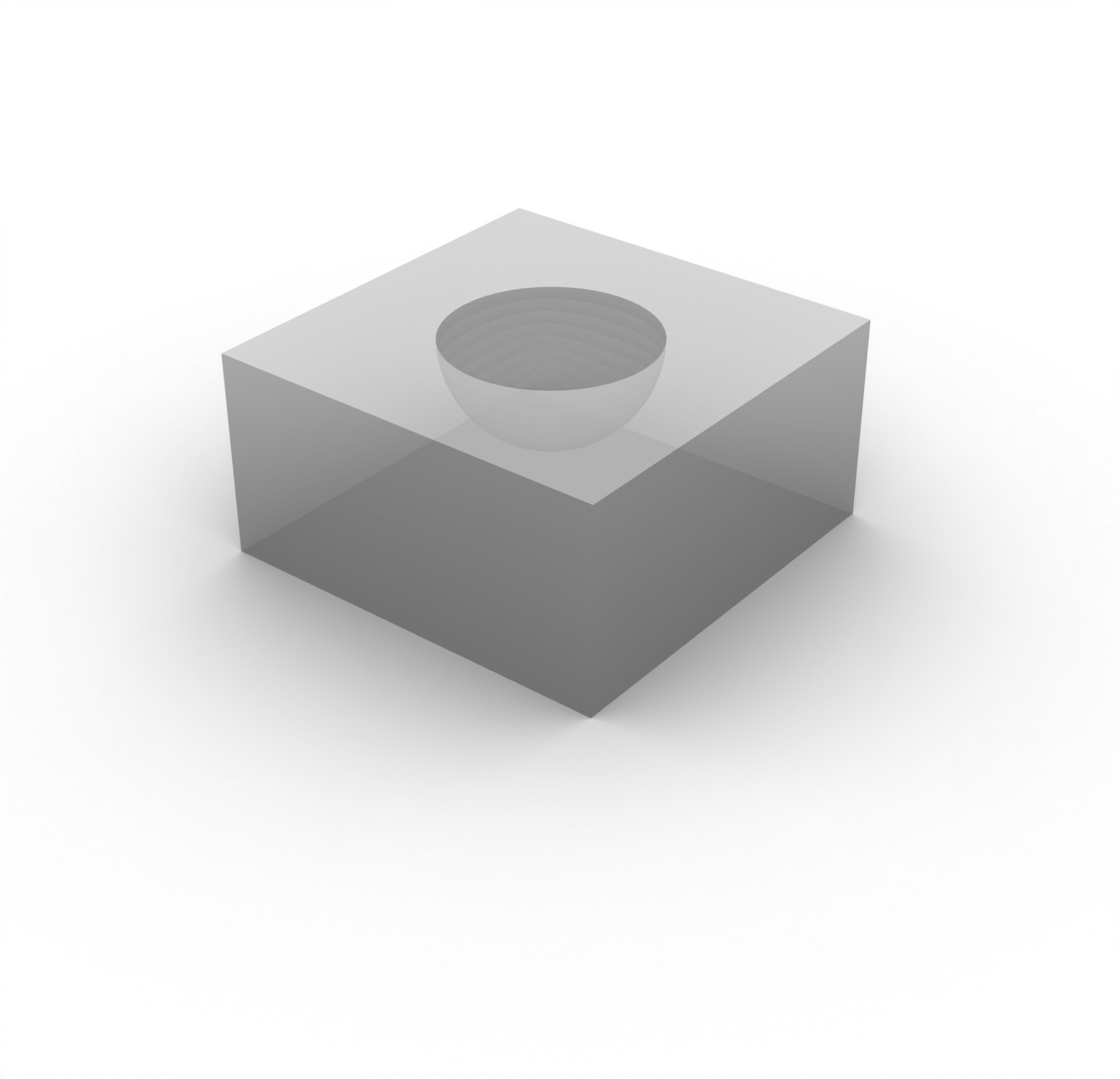
First, the base geometry consisting of a cuboid and a hemisphere will be
generated using
brick x 2 y 2 z 1 create sphere radius 0.5 move Volume 2 z 0.5 include_merged
In order to remove the part of the cuboid where it overlaps with the sphere,
a boolean subtraction can be performed with
subtract volume 2 from volume 1 keep_tool
Next, the sphere can be webcut in order to remove the upper portion of it;
this leaves behind the bottom hemisphere.
webcut volume 2  with plane from surface 9
delete volume 2
Next, overlapping surfaces are merged in order to consolidate common surface
entities using
merge surface all
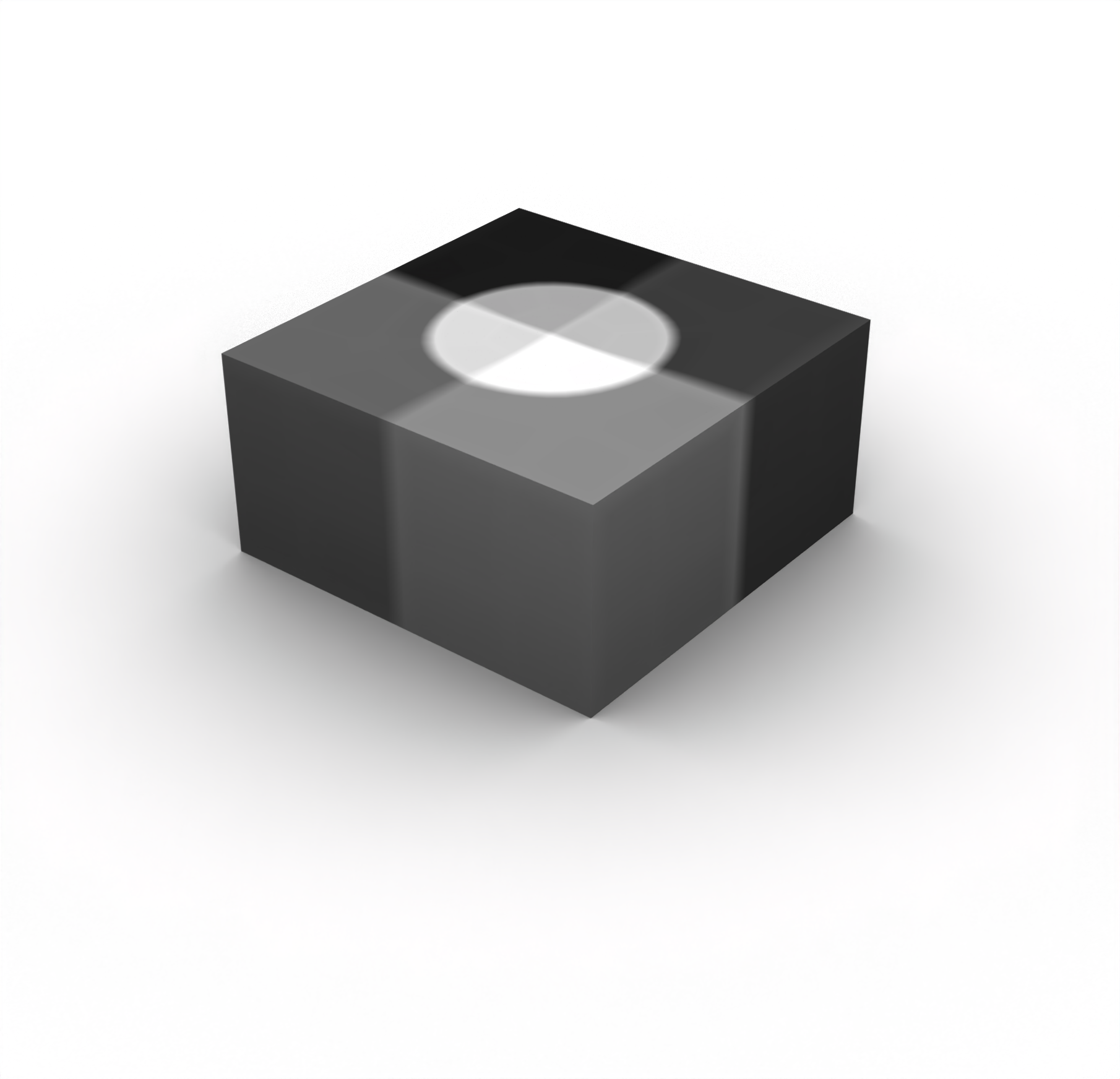
Before commencing with the meshing of the geometry, a series of webcuts need
to be applied to the geometry. These will be used in order to guide the
mesher when constructing the discretization. In particular, cutting the
geometry into quadrants through the origin in the - and -planes will
make the polyhedron meshing scheme particularly well-suited for this
geometry. This webcutting can be achieved with
webcut volume all with plane xplane offset 0
webcut volume all with plane yplane offset 0

merge surface all
As noted previously, the polyhedron meshing scheme will be applied to all of
the geometric entities with
volume all scheme polyhedron
Next, the element sizes can again be approximated using the same approach as
detailed in the 2D example. Here we will consider the following material
properties:
| Entity | Physics | VP | VS | RHO |
|---|---|---|---|---|
| Hemisphere | Acoustic | 1500 | N/A | 1000 |
| Cuboid | Elastic | 4500 | 3000 | 2000 |
We'll again discretize the domain with approximately 2.0 elements per
wavelength, but for this simulation we'll use a source frequency of 20 kHz.
This results in the approximate element sizes of
and
These element sizes can then be applied with
volume 3 5 7 9 size 0.0375
volume 1 4 6 8  size 0.075
volume 3 5 7 9  sizing function type skeleton min_size auto max_size 0.0375 max_gradient 1 min_num_layers_3d 1 min_num_layers_2d 1 min_num_layers_1d 1
volume 1 4 6 8  sizing function type skeleton min_size auto max_size 0.075 max_gradient 1 min_num_layers_3d 1 min_num_layers_2d 1 min_num_layers_1d 1
The polyhedron scheme requires all of the regions of the domain to be meshed
at once. Thus, we can simply run
mesh volume all
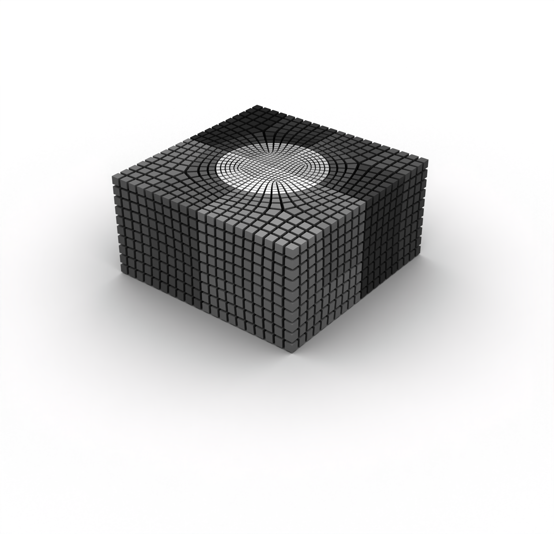
The uniformity of the elements can be improved using mesh smoothing through
the use of
surface all smooth scheme edge length
surface smooth all

volume all smooth scheme equipotential
smooth volume all
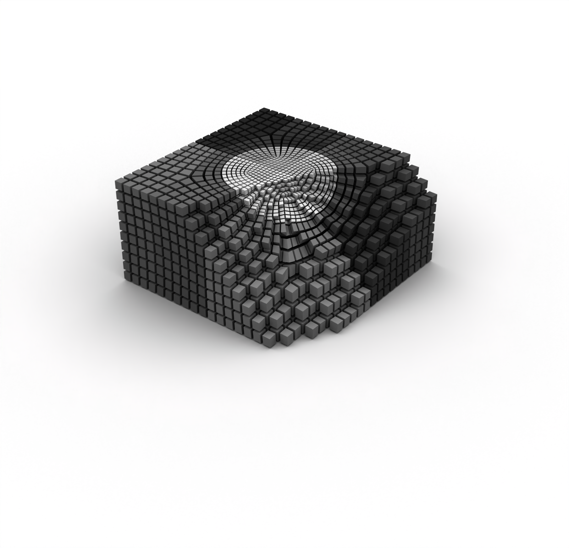
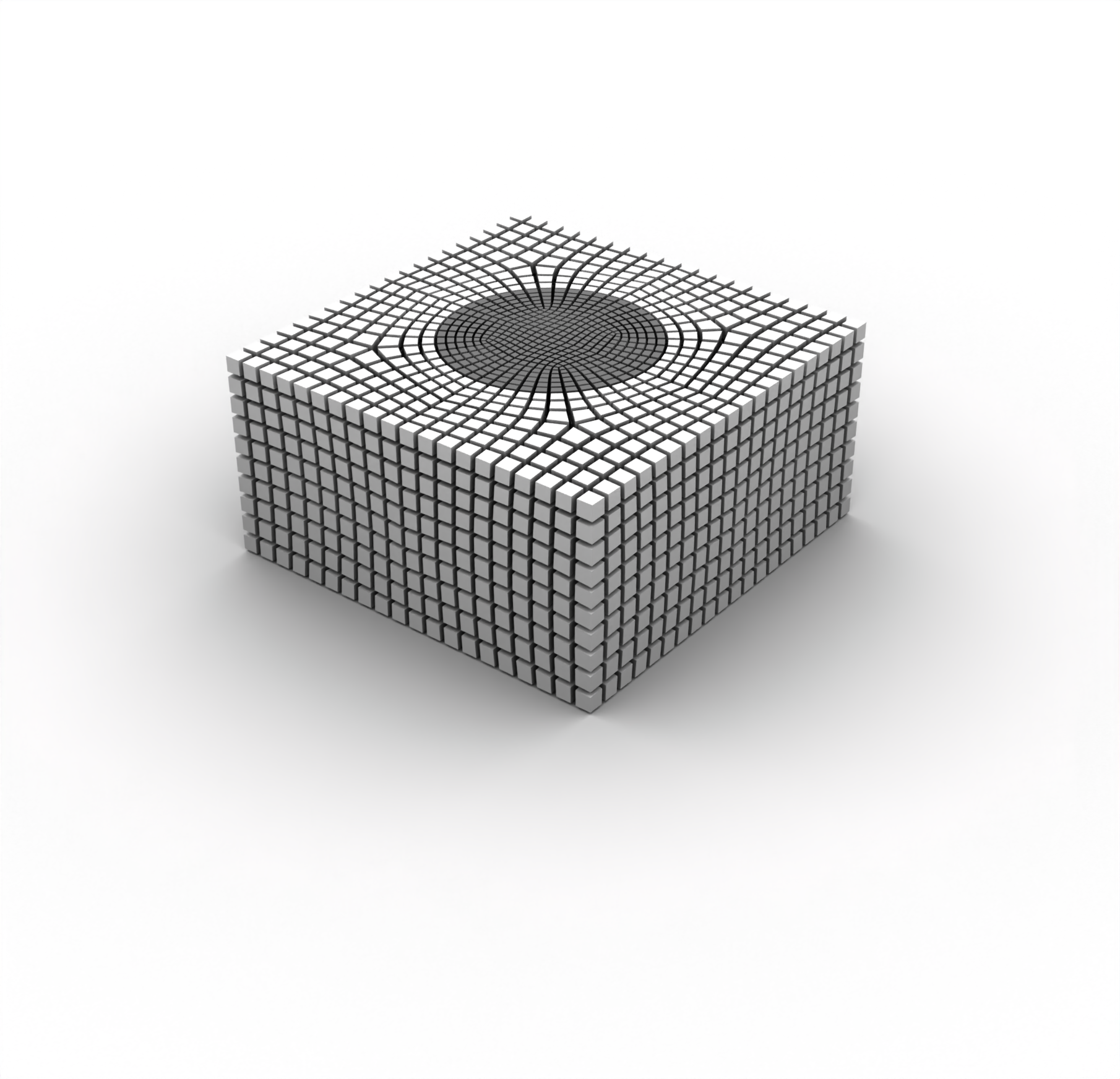
Here's what the mesh looks like, along with a cut-away to reveal its internal
structure:
Finally, each of the individual parts in the hemisphere and the cuboid can be
added to a single block; this will become useful later when attempting to
assign material properties to discrete blocks within the domain. This can be
achieved using
block 1 add volume 3 5 7 9
block 2 add volume 1 4 6 8
As before, the mesh can be exported to Exodus using
set exodus netcdf4 on
export mesh "/path/to/file/sample_3D.e" dimension 3
Similar to the 2D example, here's a complete list of the journal commands
necessary for creating the mesh:
# Create the cuboid
brick x 2 y 2 z 1

# Create the sphere and shift it upwards
create sphere radius 0.5
move Volume 2 z 0.5 include_merged

# Subtract the sphere from the cuboid
subtract volume 2 from volume 1 keep_tool

# Remove the top part of the sphere
webcut volume 2  with plane from surface 9
delete volume 2

# Combine the bowl parts of the surfaces
merge surface all

# Make webcuts so that we can use the polyhedron scheme on everything
webcut volume all with plane xplane offset 0
webcut volume all with plane yplane offset 0

# Merge the webcut surfaces
merge surface all

# Use the polyhedron scheme to mesh everything
volume all scheme polyhedron

# Set the element sizes
volume 3 5 7 9 size 0.0375
volume 1 4 6 8  size 0.075
volume 3 5 7 9  sizing function type skeleton min_size auto max_size 0.0375 max_gradient 1 min_num_layers_3d 1 min_num_layers_2d 1 min_num_layers_1d 1
volume 1 4 6 8  sizing function type skeleton min_size auto max_size 0.075 max_gradient 1 min_num_layers_3d 1 min_num_layers_2d 1 min_num_layers_1d 1

# Mesh everything
mesh volume all

# Smooth the mesh a bit
surface all smooth scheme edge length
smooth surface all
volume all smooth scheme equipotential
smooth volume all

# Assign everything as two blocks
block 1 add volume 3 5 7 9
block 2 add volume 1 4 6 8

# Export to Exodus
set exodus netcdf4 on
export mesh "/path/to/file/sample_3D.e" dimension 3
Importing meshes in 3D is extremely similar to how it is performed in 2D. In
fact, we'll re-use many of the functions we defined in the previous example
for the 3D mesh.
import os

import matplotlib.pyplot as plt
import numpy as np

from salvus.mesh.algorithms.unstructured_mesh.metrics import compute_time_step
import salvus.namespace as sn

SALVUS_FLOW_SITE_NAME = os.environ.get("SITE_NAME", "local")
RANKS_PER_JOB = 1
We can again use the
from_exodus constructor to directly import the Exodus
mesh.m_3d = sn.UnstructuredMesh.from_exodus(
"data/sample_3D.e", attach_element_block_indices=True
)
# Add a side set to the mesh so that we can visualize the mesh
m_3d.find_surface()
m_3d
<unstructured_mesh.unstructured_mesh.UnstructuredMesh object at 0x70b7c256b250>
We can re-use the same material properties dictionary as we used in the
previous tutorial:
# Define our properties for the mesh
block_props = {
    1: {"VP": 1500.0, "RHO": 1000.0},
    2: {
        "VP": 4500.0,
        "VS": 3000.0,
        "RHO": 2000.0,
    },
}
Let's apply the materials and perform the mesh QC.
def assign_properties_to_mesh(
    mesh: sn.UnstructuredMesh, properties: dict
) -> None:
    # Initialize the fluid flag
    mesh.attach_field("fluid", np.zeros(mesh.nelem, dtype=bool))

    # Initialize the elemental fields for the mesh
    for field in ["VP", "VS", "RHO"]:
        mesh.attach_field(field, np.zeros_like(mesh.connectivity, dtype=float))

    for block_id in properties:
        # Get the elements that belong to the given block ID
        mask = mesh.elemental_fields["element_block_index"] == block_id

        # Assign the material properties for that block
        for field, value in properties[block_id].items():
            mesh.elemental_fields[field][mask, :] = value

        # Set the fluid flag for the given block; this will tell the solver
        # whether to use the acoustic or elastic solver for that part of the
        # mesh
        if "VS" not in properties[block_id]:
            mesh.elemental_fields["fluid"][mask] = True
        else:
            mesh.elemental_fields["fluid"][mask] = False


assign_properties_to_mesh(m_3d, block_props)
m_3d.qc_test()
[2026-05-01 14:23:08,767] INFO: [SUCCESS] No issues found!
{}Everything there looks good, so let's again proceed to looking at the
resolved frequencies and the global time step that the mesh is able to
obtain.
As within the 2D example, let's compute the minimum resolved frequencies and
the global time step that the mesh is able to achieve.
min_velocity = np.zeros(m_3d.nelem, dtype=float)

for block_id, props in block_props.items():
    mask = m_3d.elemental_fields["element_block_index"] == block_id

    if "VS" in props:
        min_velocity[mask] = np.min(
            m_3d.elemental_fields["VS"][mask, :], axis=1
        )
    else:
        min_velocity[mask] = np.min(
            m_3d.elemental_fields["VP"][mask, :], axis=1
        )

min_frequency_3d, resolved_frequencies_3d = m_3d.estimate_resolved_frequency(
    min_velocity=min_velocity,
    elements_per_wavelength=2.0,
)

print("Minimum resolved frequency is %.2f kHz" % (min_frequency_3d / 1e3))
Minimum resolved frequency is 14.76 kHz
The minimum resolved frequency is somewhat below our desired bound of 20kHz.
This implies that there are some elements in the mesh that are larger than we
might like, which might cause us to accumulate more numerical dispersion as a
result. Let's take a look at the resolved frequencies for the mesh:
def colored_histogram(
    data: np.ndarray,
    n_bins: int = 50,
    colormap: str = "coolwarm",
) -> None:
    counts, bins = np.histogram(data, bins=n_bins)

    fig = plt.figure(figsize=[10, 3])
    cmap = plt.get_cmap(colormap)
    colors = cmap(np.linspace(0, 1, len(bins) - 1))

    for i in range(len(bins) - 1):
        plt.bar(
            bins[i],
            counts[i],
            width=bins[i + 1] - bins[i],
            color=colors[i],
            edgecolor="black",
        )

    return fig, counts, bins


def plot_resolved_frequencies(
    resolved_frequencies: np.ndarray,
    n_bins: int = 50,
    colormap: str = "coolwarm",
) -> None:
    _, counts, bins = colored_histogram(
        resolved_frequencies / 1e3, n_bins, colormap
    )

    plt.annotate(
        "Elements\nToo Large",
        xy=(bins[0], max(counts) * 0.45),
        xytext=(bins[6], max(counts) * 0.45),
        arrowprops=dict(facecolor="black", arrowstyle="-|>", lw=1.5),
        ha="center",
        va="center",
    )
    plt.annotate(
        "Elements\nToo Small",
        xy=(bins[-1], max(counts) * 0.45),
        xytext=(bins[-7], max(counts) * 0.45),
        arrowprops=dict(facecolor="black", arrowstyle="-|>", lw=1.5),
        ha="center",
        va="center",
    )

    plt.title("Resolved Frequencies")
    plt.xlabel("Frequency [kHz]")
    plt.ylabel("Number of Elements")
    plt.show()


def plot_dt(
    dts: np.ndarray, n_bins: int = 50, colormap: str = "coolwarm_r"
) -> None:
    _, counts, bins = colored_histogram(dts, n_bins, colormap)

    plt.annotate(
        "Restricting\nTime Step",
        xy=(bins[0], max(counts) * 0.05),
        xytext=(bins[0], max(counts) * 0.3),
        arrowprops=dict(facecolor="black", arrowstyle="-|>", lw=1.5),
        ha="center",
        va="center",
    )

    plt.title("Time Steps")
    plt.xlabel(r"$\Delta t$ [$\mu$s]")
    plt.ylabel("Number of Elements")
    plt.show()


plot_resolved_frequencies(resolved_frequencies_3d)
It appears that most of the elements are, indeed, slightly below the desired
bound of 20kHz. This means that we would ideally choose to mesh the domain
with a slightly finer discretization in order to avoid the presence of these
large elements. It is generally helpful to plot the resolved frequencies in
order to identify the problematic elements in the mesh:
m_3d.attach_field("resolved_frequency", resolved_frequencies_3d)

# Change plotted field to `resolved_frequency`
m_3d
<unstructured_mesh.unstructured_mesh.UnstructuredMesh object at 0x70b7c256b250>
Note that here we are only plotting the elements on the surface of the
hexahedral mesh; one could use the
write_h5() method in order to visualize
the internal structure of the mesh in an alternative visualization tool such
as ParaView.The tail on the right-hand-side of the resolved frequencies histogram implies
that the mesh also contains some locally constricted elements, given that the
upper bound of the resolved frequencies is higher than the expected maximum
frequency of the source. This suggests that the time step will likely become
limited by a handful of these small elements.
To verify that this is indeed the case, let's compute the time steps of each element.
dt_3d, dts_3d = compute_time_step(
    mesh=m_3d,
    max_velocity=m_3d.elemental_fields["VP"].max(axis=1),
)

print(f"Global time step: {dt_3d * 1e6:.2f} us")

plot_dt(dts_3d * 1e6)
Global time step: 0.40 us

We can see in this distribution of the time steps across all of the elements
in the mesh that there are a handful of elements that are restricting the
time step. Let's plot the on the mesh so that we can see the
parts of the discretization that are problematic for the time step.
m_3d.attach_field("dt", dts_3d)

# Change plotted field to `dt`
m_3d
<unstructured_mesh.unstructured_mesh.UnstructuredMesh object at 0x70b7c256b250>
At this stage, one could return to the meshing stage in order to improve the
quality of the discretization. However, for the sake of this example, we
will proceed with the existing mesh that we have, but with the understanding
that further improvements to the mesh could be conducted.
Let's again set up a very minimalistic forward simulation to demonstrate that
this mesh actually works in a wave simulation:
p_3d = sn.Project.from_mesh(
    path="project_3D",
    mesh=m_3d,
    load_if_exists=True,
)

p_3d.add_to_project(
    sn.Event(
        event_name="event_3D",
        sources=sn.simple_config.source.cartesian.ScalarPoint3D(
            x=0.0, y=0.0, z=0.5, f=1.0
        ),
    )
)

wsc = sn.WaveformSimulationConfiguration(end_time_in_seconds=500.0e-6)
stf = sn.simple_config.stf.Ricker(center_frequency=20e3 / 2)
stf.plot()
p_3d.add_to_project(
    sn.UnstructuredMeshSimulationConfiguration(
        name="forward_simulation_3D",
        unstructured_mesh=m_3d,
        event_configuration=sn.EventConfiguration(
            waveform_simulation_configuration=wsc,
            wavelet=stf,
        ),
    )
)
Before running the simulation, we'll double check the simulation setup:
p_3d.viz.nb.simulation_setup(
    simulation_configuration="forward_simulation_3D",
    events="event_3D",
)
<salvus.flow.simple_config.simulation.waveform.Waveform object at 0x70b7b9cc5210>
That looks good to go! A few small things to note here about this simulation:
- We'll only output a very small number of time steps (i.e., with
sampling_interval_in_time_steps) in order to keep the file size of the wavefield small. If you would want to create a wavefield animation for this data, decreasing thesampling_interval_in_time_stepswould output more time steps. However, be warned that the files can quickly become very large! - Increasing the number of ranks in accordance with the number of CPU cores that your machine has will make the simulation run much more quickly.
p_3d.simulations.launch(
    simulation_configuration="forward_simulation_3D",
    events="event_3D",
    site_name=SALVUS_FLOW_SITE_NAME,
    ranks_per_job=RANKS_PER_JOB,
    extra_output_configuration={
        "volume_data": {
            "sampling_interval_in_time_steps": 1000,
            "fields": ["displacement", "gradient-of-phi"],
        },
    },
)
[2026-05-01 14:23:10,760] INFO: Submitting job ... Uploading 1 files... 🚀 Submitted job_2605011423831691_ecf3ecdf2c@local
1
p_3d.simulations.query(
    simulation_configuration="forward_simulation_3D",
    events="event_3D",
    block=True,
)
True
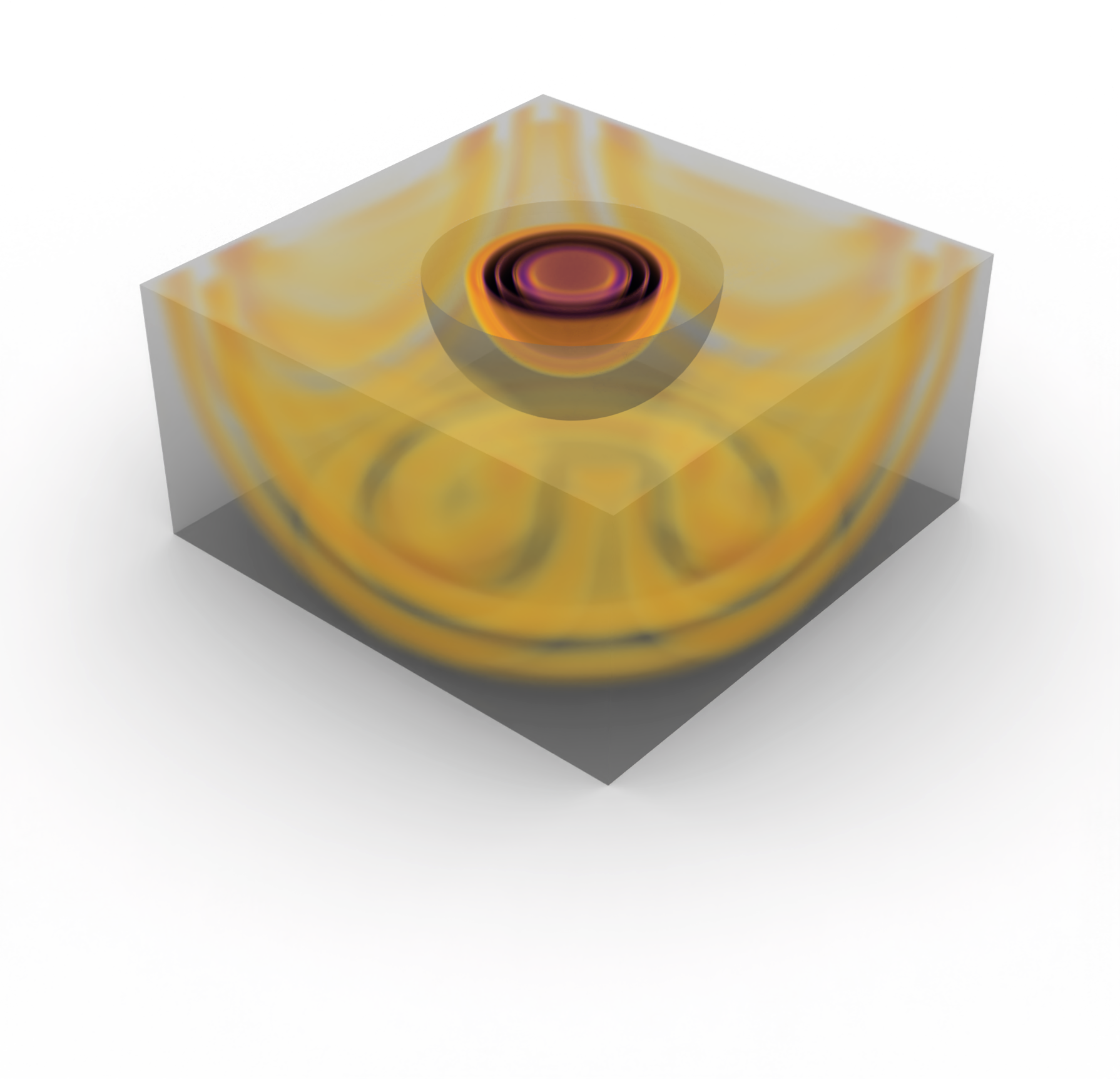
Finally, we can again visualize the wavefield data in a visualization
software such as ParaView. As with the 2D example, the relevant state file
is provided in order to plot this wavefield in ParaView. Here is a snapshot
of the final time step of the wavefield:

PAGE CONTENTS