Salvus 0.11.41

The observed and synthetic data can now optionally be downsampled before the misfit and adjoint source are computed. The adjoint source is later upsampled again and scaled correctly. Useful for expensive misfit functionals.

It can be used either at the event misfit level:

event_misfit = EventMisfit(
    ...,
    # Optionally downsample to the given number of npts.
    max_samples_for_misfit_computation=max_samples_for_misfit_computation
)

Or at the misfit configuration level within SalvusProject:

mc = MisfitConfiguration(
    ...,
    # Optionally downsample to the given number of npts.
    max_samples_for_misfit_computation=max_samples_for_misfit_computation

Fix a bug that caused the mesh widget to crash for fields with only negative values.

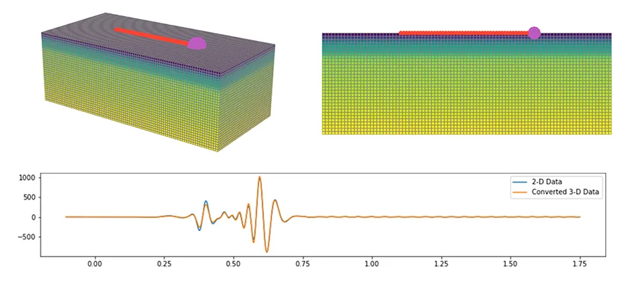
Added comprehensive support for converting data from a point source to an equivalent line source which is necessary for example when using 3-D observed data in 2-D inversions.

We added a variety of different transform, each applicable in different use cases. Please have a look at the documentation for details.

from salvus.modules.near_surface.processing import convert_point_to_line_source

new_st = convert_point_to_line_source(
    st=st,
    source_coordinates=[22.0, 1.0],
    receiver_coordinates=[132.0, 0.0],
    transform_type="single_velocity_exact",
    velocity_m_s=550.0
)

Added utility functions to compute, remove, and plot geophone responses.

import numpy as np
from salvus.modules.near_surface.processing import geophone_response

frequencies = np.logspace(0.1, 2, 2000)
response = geophone_response.compute_geophone_response(
    frequencies=frequencies,
    geophone_frequency=4.5,
    damping_ratio=0.4,
    calibration_factor=11.2,
)
geophone_response.plot_response(frequencies=frequencies, response=response)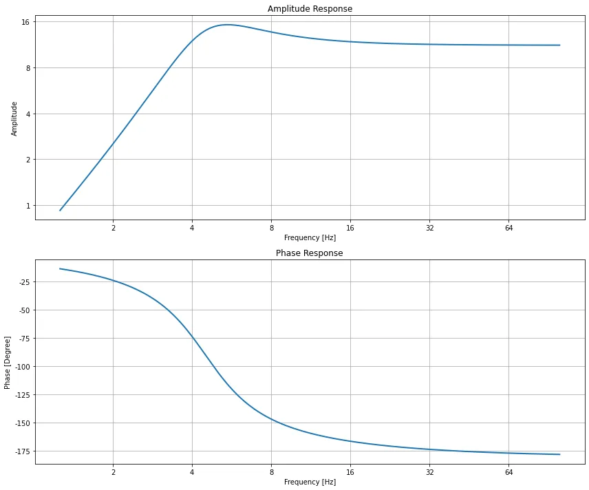

Added an implementation of a graph space optimal transport misfit measure as introduced in this paper:

L. Métivier, R. Brossier, Q. Mérigot, and E. Oudet. 2019.

“A graph space optimal transport distance as a generalization of Lp  distances: application to a seismic imaging inverse problem”

Inverse Problems, Volume 35, Number 8, https://doi.org/10.1088/1361-6420/ab206f

You can use it by choosing "graph_space_optimal_tranport" everywhere Salvus accepts misfit functionals. The one tuning parameters is the "max_expected_time_shift" which, as the name implies, should be set to the maximum expected time shift in seconds for individual wiggles between observed and synthetic data.

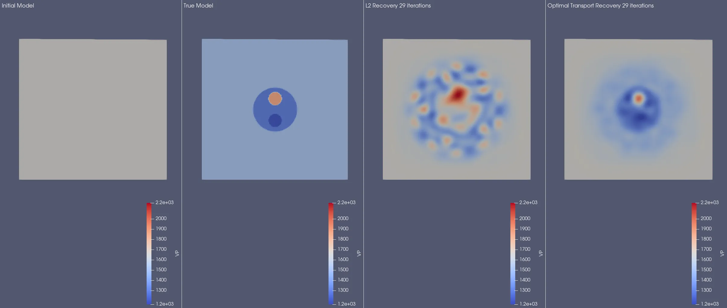
For many problems this can get completely avoid the cycle skipping problem. This, admittedly manufactured, synthetic inversion example demonstrates the potential gains:

The function serialization can now serialize numpy arrays and dictionaries as closure values.

Added the ability to use processing fragments to more easily perform some simple and common processing techniques.

To for example bandpass and normalize some data use "EXTERNAL_DATA:raw_data | bandpass(1.0, 2.0) | normalize" as the data name.

Available processing fragments:

• time_shift({SHIFT})
• normalize
• scale({FACTOR})
• flip
• bandpass({FREQ_MIN}, {FREQ_MAX}[, zerophase][, corners={CORNERS}])

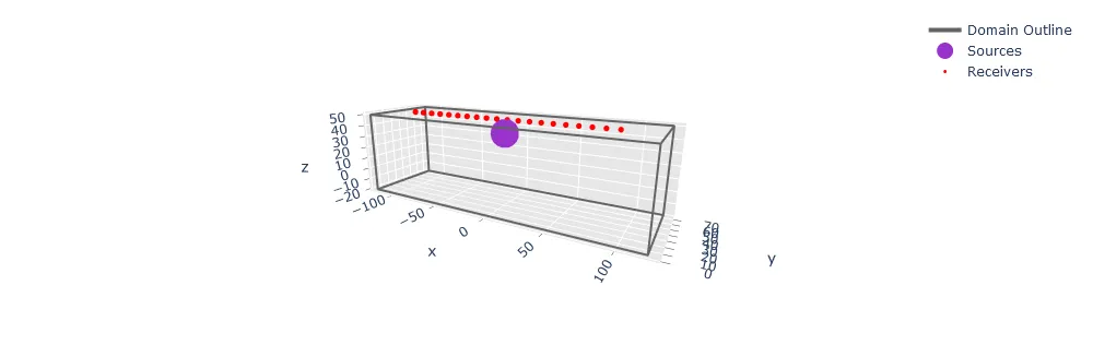
Added an automatic domain preview visualization for 3-D box domains.

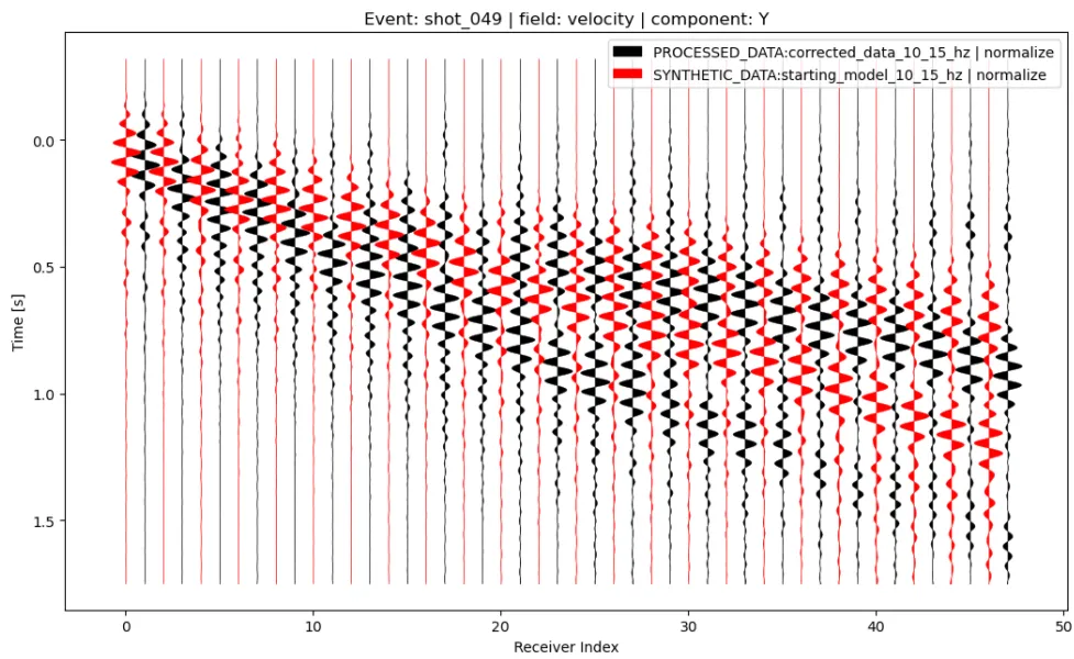
Added an improved shotgather visualization. Amongst other things, it can now plot interleaved data from multiple traces and sort the receivers with a lambda function:

p.viz.shotgather(
    data=[
        "PROCESSED_DATA:corrected_data_10_15_hz | normalize",
        "SYNTHETIC_DATA:starting_model_10_15_hz | normalize",
    ],
    event="shot_049",
    receiver_field="velocity",
    component="Y",
    sort_by=lambda r: r.location[0]
)

Allow for the passing of an interpolation mode to the mesh_from_xarray function in the Salvus Toolbox. This allows one to override the default spline interpolation routine, which may be useful in the presence of strong velocity contrasts.