Mondaic - Full Waveform Solutions

In this guide, we will learn how to add measured data to a Salvus project. We will then run some simulations by building a digital twin of the real-world experiment and compare the actually measured data with simulated data. The example that we will look at here is concerned with ultrasonic inspection. We will use a reference ultrasonic dataset recorded on a polyamide block specimen with a simple geometry. The simplicity of the experiment highly facilitates the interpretation of the data. The dataset is described in detail in the paper Maack et al. (2022), Low frequency ultrasonic dataset for pulse echo object detection in an isotropic homogeneous medium as reference for heterogeneous materials in civil engineering. The full dataset is published open-access under the Creative Commons license and can be downloaded here. To keep the computational costs tractable, we will look at a select few shots out of the dataset.

By the end of this tutorial, you will:

Know how you can add your own measurement data to a Salvus project.
Know how to use the Salvus internal waveform retrieval functionality to plot comparisons between observed and simulated data.
Have learned how you can simulate data of (phased-)array transducer ultrasonic probes.
Have observed how Salvus simulations in a digital twin can match real-world experimental data 'wiggle-by-wiggle'.

The polyamide block specimen used in the experimental data looks like this (Figure reproduced after Figure 5 in Maack et al. (2022)).

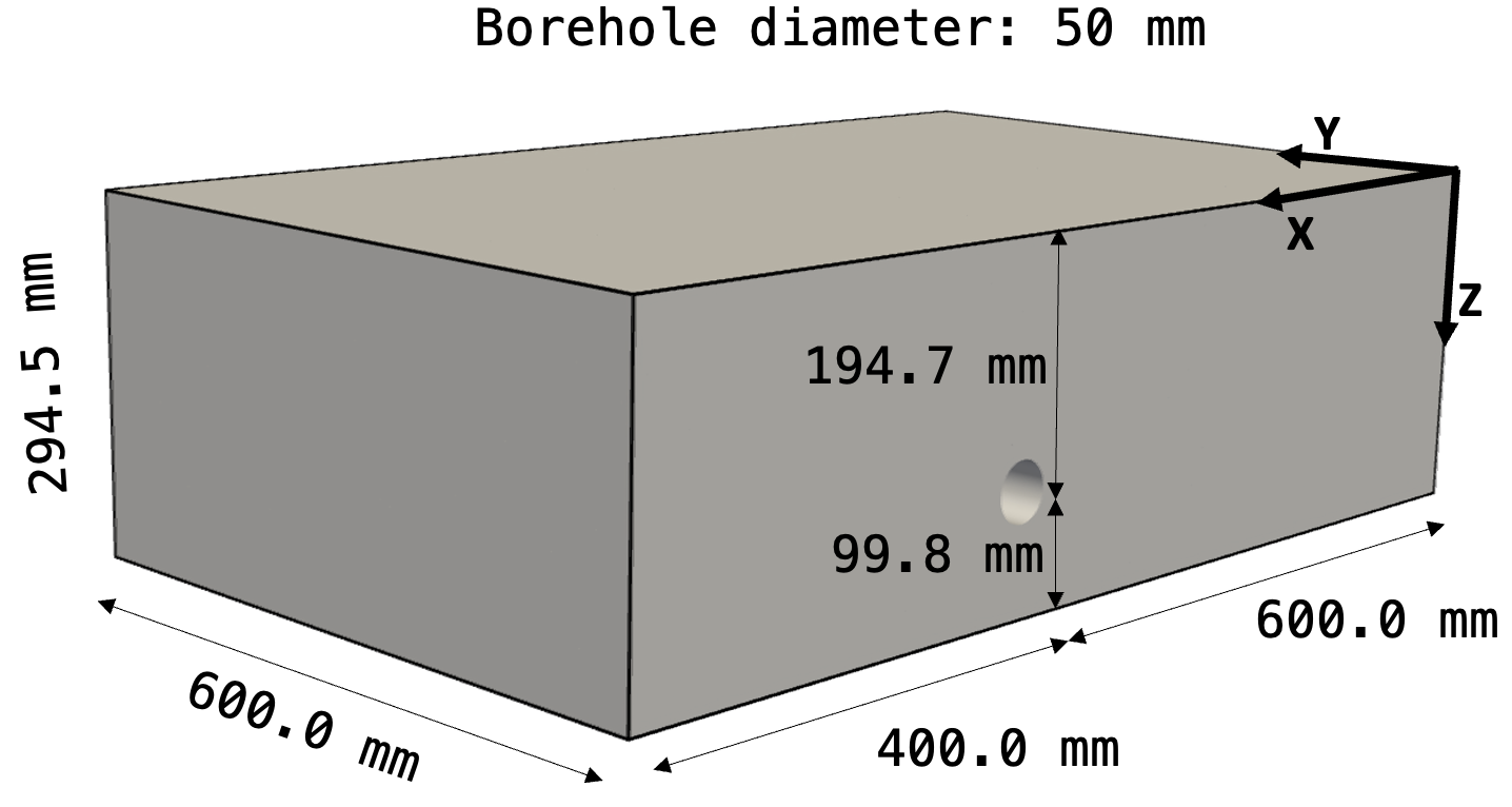
As you can see, the test block contains a single borehole with a diameter of 50 mm. The experimental data was recorded in the coordinate frame depicted by the bold arrows with the origin in the top right corner. We now want to use Salvus to simulate ultrasonic data in a digital twin of this test block and compare it to the actually recorded data.

As always, we first import some of the Python packages that we need to run this example.

import os

import matplotlib.pyplot as plt
import numpy as np
import xarray as xr

import salvus
import salvus.namespace as sn

SALVUS_FLOW_SITE_NAME = os.environ.get("SALVUS_FLOW_SITE_NAME", "local")

Let us start by setting up a Salvus project from a simulation domain where we set up the dimension object from the measures of the test body given in the figure above. Note that, following Salvus coordinate conventions, the x- and z-axes are flipped compared to the coordinate frame that the measurements are defined in.

domain = sn.domain.dim3.BoxDomain(
    x0=0.0,
    x1=1.0,
    y0=0.0,
    y1=0.6,
    z0=-0.2945,
    z1=0.0,
)

p = sn.Project.from_domain(
    path="project",
    domain=domain,
    load_if_exists=True,
)

domain.plot()

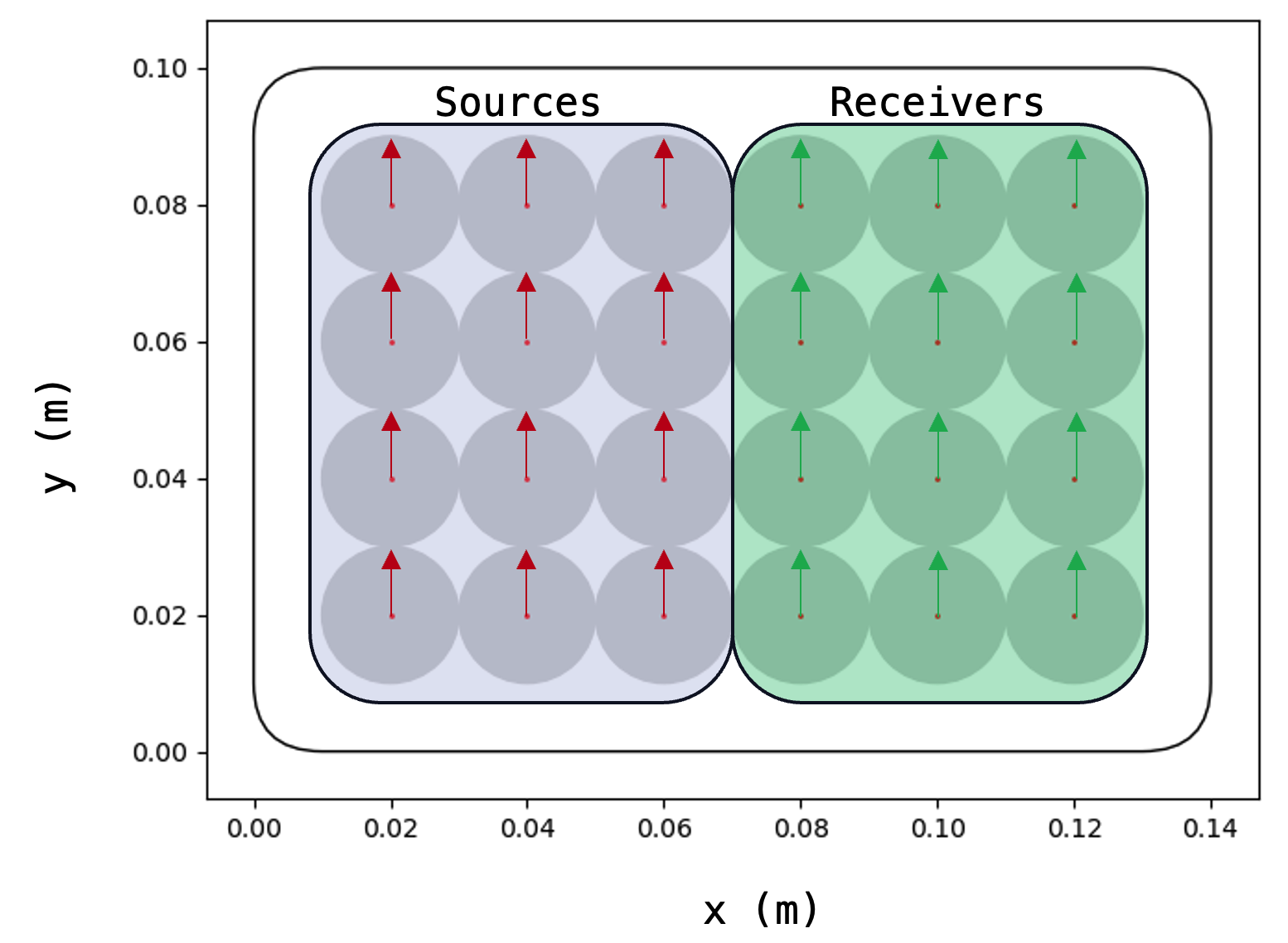
The data were recorded with an ultrasonic probe that includes 24 transducer elements. From the 24 transducers, 12 are simultaneously excited as sources and 12 are parallel-connected as receivers. This means that the signals recorded by the 12 receivers are internally summed up to yield a single output signal at each probe location.

Here we provide a view from the bottom of the probe where the small arrows inside each transducer element indicate that the probe was run in Shear-wave mode, meaning that transverse waves are excited in the direction of the arrow at the source positions and the corresponding direction of particle displacement is recorded at the receiver positions.

Now, let us load some of the measurement data. With this tutorial, we provide the comma-separated file 'data/Shear_x001-x101_y025_Rot00.csv', which contains a single line profile of data. Of course, please feel free to download other profiles directly from the source. To acquire the line of data, the probe was moved across the surface of the specimen in 10 mm increments in the x-direction. Such line measurements are typically referred to as "B-scans". Each of the 100 columns of the dataset thus corresponds to a single measurement position (indexed from 'x001 = 0 m' to 'x101 = 1 m'). The profile was located at a lateral position of 'y025=0.24 m'. For the B-scan included in this tutorial, the probe was oriented in the following way (after Maack et al., 2022):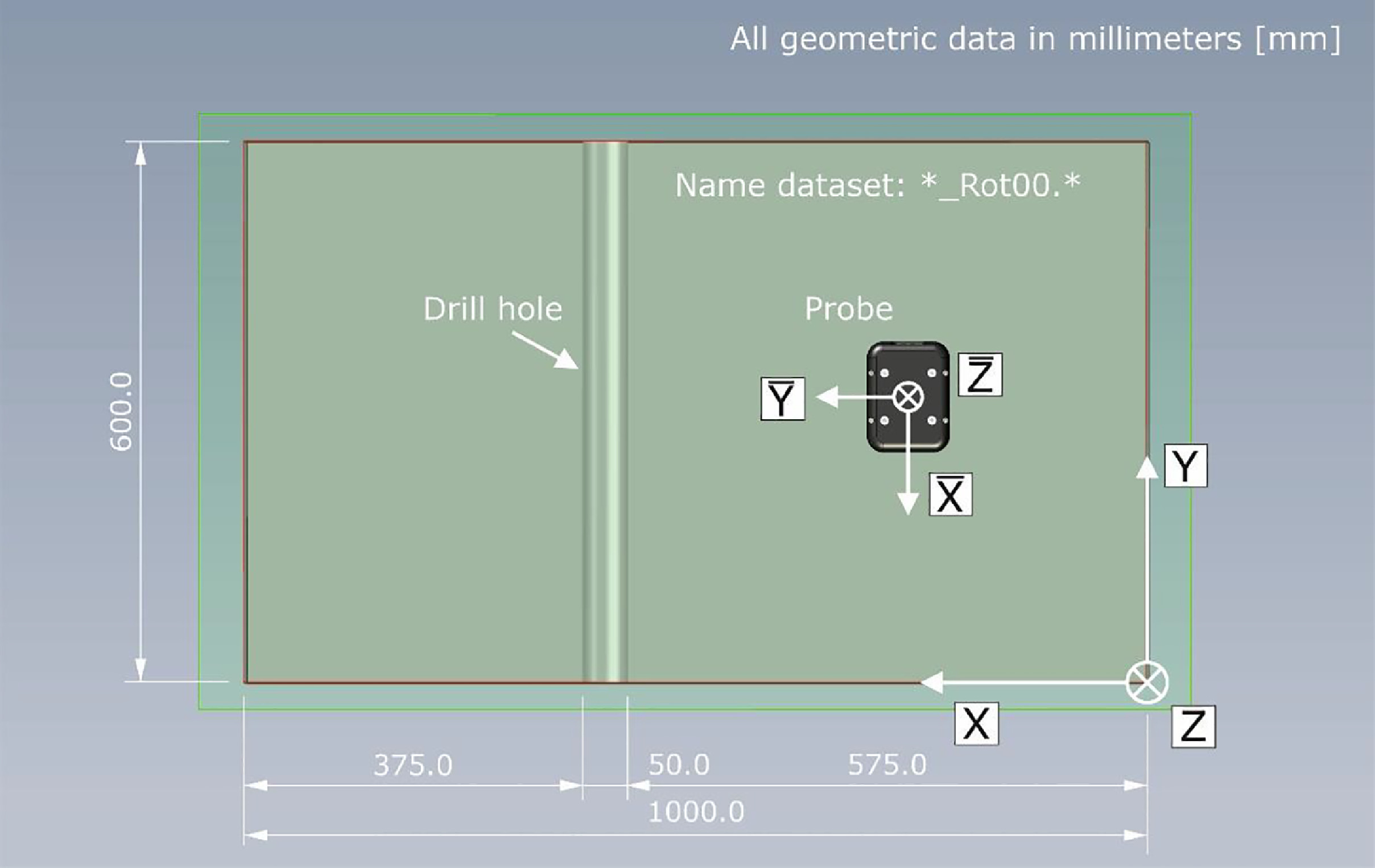

# Load the data from the CSV file
data = np.genfromtxt("data/Shear_x001-x101_y025_Rot00.csv", delimiter=",")
sampling_rate_in_hz = 2_000_000  # The data is sampled at 2 Mhz
dx = 0.01  # X-spacing of measurement positions
t = np.arange(data.shape[1]) * (1 / sampling_rate_in_hz)  # The time axis
x = np.arange(data.shape[0]) * dx
y = 0.24  # Profile at y=0.24m
z = 0.0  # Measurements are taken at the surface at z=0m

For visualization, we now wrap this data into an xarray.DataArray object with an 'x' and 'time' coordinate, which provides us with a nice way to store and plot structured data. We can already see some interesting features in the data:

The direct wave close to t=0 seconds.
The reflection off the bottom of the specimen at t~=5.5e-3 seconds and multiples thereof.
The diffraction hyperbola of the borehole with the apex located at x=0.6 m.

observed_data = xr.DataArray(
    data=data, dims=["x", "time"], coords={"x": x, "time": t}
)
observed_data.T.plot()

<matplotlib.collections.QuadMesh at 0x7a31561507d0>

To perform data-fusion, we now would want to run Salvus simulations for the same line of data. First, we define the material parameters of the polyamide block. We have done some calibration of the material properties for you and found the following properties to be a good representation of the physical properties of the block:

P-wave velocity: 1990 m/s
S-wave velocity: 1136 m/s
Density: 1150 kg/m^3

In practice, you could of course use Salvus' full waveform inversion capabilities to calbirate the material properties, but this is beyond the scope of this example. The polyamide is also dissipative, so we will run a visco-elastic simulation with the following attenuation parameters:

Q factor for the bulk modulus: 85 m⁻¹
Q factor for Lame's second parameter: 85 m⁻¹

Please refer to the attenuation tutorial for more information on running viscoacoustic and viscoelastic simulations with Salvus.

From these properties, we set up a homogeneous model.

parameters = {
    "VP": 1990.0,  # P-wave velocity (m/s)
    "VS": 1136.0,  # S-wave velocity (m/s)
    "RHO": 1150.0,  # Density (kg/m^3)
    "QKAPPA": 85.0,  # Q for the bulk modulus.
    "QMU": 85.0,  # Q for Lame's second parameter (mu).
}

mc = sn.ModelConfiguration(
    background_model=sn.model.background.homogeneous.IsotropicViscoElastic(
        vp=parameters["VP"],
        vs=parameters["VS"],
        rho=parameters["RHO"],
        qkappa=parameters["QKAPPA"],
        qmu=parameters["QMU"],
    ),
    linear_solids=sn.LinearSolids(reference_frequency=60_000),
)

Now, we need to create Salvus Event objects for each measurement position on our profile, where an Event corresponds to a digital twin of the probe transducer locations at a specific measurement position. So, let us first specify some general geometrical properties of the probe.

transducer_dx = 0.02  # Transducer spacing in x-direction
transducer_dy = 0.02  # Transducer spacing in y-direction
nx = 4  # Number of transducers in x direction for given probe orientation
ny = 6  # Number of transducers in y-direction for given probe orientation
transducer_x = np.arange(nx) * transducer_dx
transducer_y = np.arange(ny) * transducer_dy
X, Y = np.meshgrid(
    transducer_x, transducer_y
)  # XY Coordinates for each transducer
X, Y = X.ravel() - np.mean(transducer_x), Y.ravel() - np.mean(
    transducer_y
)  # Place the center of the instrument at the origin

# Split into sources and receivers
x_sources = X[Y > 0]
y_sources = Y[Y > 0]
x_receivers = X[Y < 0]
y_receivers = Y[Y < 0]

# A quick plot of the transducer coordinates for QC
plt.figure()
plt.plot(x_sources, y_sources, "b.", label="sources")
plt.plot(x_receivers, y_receivers, "g.", label="receivers")
plt.gca().set_aspect("equal")
plt.xlabel("X (m)")
plt.ylabel("Y (m)")
plt.title("Transducer locations")
plt.legend()

<matplotlib.legend.Legend at 0x7a3156181710>

Now we define the Events for each measurement position by moving the coordinates our device to the position of the measurements and defining the corresponding sources and receivers. We do offer a digital twin library for a series of commercially available ultrasonic probes that facilitates the creation of these events. However, in this tutorial, we show how this can be done manually in order to facilitate adapting your workflow to arbitrary probe geometries.

for i, pos_x in enumerate(x):
    event = sn.Event(
        event_name=f"event{i+1:03d}",
        sources=[
            sn.simple_config.source.cartesian.VectorPoint3D(
                x=1.0 - (sx + pos_x),  # Account for the flipped x-axis
                y=sy + y,
                z=z,
                fx=-1.0,  # Horizontally oriented source, negative X-direction
                fy=0.0,
                fz=0.0,
            )
            for (sx, sy) in zip(x_sources, y_sources)
        ],
        receivers=[
            sn.simple_config.receiver.cartesian.Point3D(
                x=1.0 - (rx + pos_x),
                y=ry + y,
                z=z,
                network_code="XX",
                station_code=f"AA{n:03d}",
                fields=["displacement"],
            )
            for n, (rx, ry) in enumerate(zip(x_receivers, y_receivers))
        ],
        # The concept of ReceiverChannel objects is described in the cell below
        receiver_channels=[
            sn.ReceiverChannel(
                identifier="OUT",
                input_receivers=[
                    f"XX.AA{n:03d}." for n in range(len(x_receivers))
                ],
                input_receiver_weights=np.ones_like(x_receivers),
                input_receiver_delays=None,
            )
        ],
    )
    try:
        p.add_to_project(event)
    except ValueError:
        # For some recording positions, the transducers would be located
        # outside the domain. We do not consider these events here.
        print(
            f"event{i+1:03d} was not added to the project as some of the "
            "sources and receivers lie outside the domain!"
        )

event001 was not added to the project as some of the sources and receivers lie outside the domain!
event002 was not added to the project as some of the sources and receivers lie outside the domain!
event003 was not added to the project as some of the sources and receivers lie outside the domain!
event099 was not added to the project as some of the sources and receivers lie outside the domain!
event100 was not added to the project as some of the sources and receivers lie outside the domain!
event101 was not added to the project as some of the sources and receivers lie outside the domain!

Note that in addition to the source and receiver objects, we have set up a ReceiverChannel object for each Event. Salvus ReceiverChannel's are a convenient way to handle parallel-connected receivers, such as the ones of our ultrasonic inspection probe. When we access the data later on, Salvus will automatically form a weighted sum of the data of the 12 receivers to combine them into a single output channel. A ReceiverChannel object takes the following input arguments:

identifier: A unique string that identifies the channel. Here, we simply used the identifier "OUT".
input_receivers: A list of the receiver names that will be combined into a single output channel.
input_receiver_weights: An array of the same length as input_receivers that specifies the relative weight that each receivers gets in the weighted sum output. In this example, we give each receiver the same weight.
input_receiver_delays: An optional array of the same length as input_receivers that specifies a time delay in seconds by which the signal of each receiver is shifted before forming the weighted sum. This can be useful when you want to simulate data of phased-array probes. In this example, we do not specify any time delays.

We are now almost ready to run some simulations. What is still missing is the source time function of the probe (i.e., the pulse that the sources transmit). Here, we provide a calibrated source time function that is close to the actual pulse emitted by the probe. The source time function is stored in "/data/stf.h5". Let us load and inspect it.

stf = sn.simple_config.stf.Custom(filename="data/stf.h5", dataset_name="stf")
stf.plot()

We now have all the information that we need to set up our simulation! We will simulate 0.001 seconds of data in a viscoelastic setup. The mesh is resolved with 1.3 elements per wavelength at a maximum frequency of 60kHz.

ec = sn.EventConfiguration(
    wavelet=stf,  # The source time function
    waveform_simulation_configuration=sn.WaveformSimulationConfiguration(
        end_time_in_seconds=0.001,  # Total simulation time,
        attenuation=True,  # We want to run a visco-elastic simulation
    ),
)

# Combine everything into a complete configuration.
p += sn.SimulationConfiguration(
    name="simulation",
    elements_per_wavelength=1.3,
    max_frequency_in_hertz=60_000,
    model_configuration=mc,
    event_configuration=ec,
)

Let us verify that we have set up everything properly. We only visualize two events (measurement positions) here. One at the very beginning of the profile and one right above the location of the borehole.

p.viz.nb.simulation_setup(
    simulation_configuration="simulation",
    events=["event015", "event061"],
)

[2025-05-21 03:01:32,806] INFO: Creating mesh. Hang on.

<salvus.flow.simple_config.simulation.waveform.Waveform object at 0x7a31560358d0>

This looks alright, so let us launch the simulations for these two events! The simulations are relatively expensive in 3D, so ideally, we would run them on a GPU.

p.simulations.launch(
    simulation_configuration="simulation",
    events=["event015", "event061"],
    site_name=SALVUS_FLOW_SITE_NAME,
    ranks_per_job=4,
)
p.simulations.query(block=True)

[2025-05-21 03:01:34,644] INFO: Submitting job array with 2 jobs ...

True

Once the simulation runs are completed, we can retrieve the simulated data for these two events from our project. Here, we directly retrieve the data as xarray.DataArray objects If you are not familiar with xarray.DataArray objects, please refer to our structured data tutorial. Note that get_waveform_data_xarray() automatically detects that our event contains a ReceiverChannel object and only returns the summed data for the receiver channel "OUT" rather than returning the data of the 12 individual receivers. We only select the "X" component of the data here as this is the only component that is measured by our ultrasonic probe given the probe orientation. For the necessity of the specific xarray's functions used, it is strongly suggested to also follow the xarray.DataArray tutorial.

edc = p.waveforms.get(
    "SYNTHETIC_DATA: simulation | normalize", events=["event015", "event061"]
)
data_event015 = (
    edc["event015"]
    .get_waveform_data_xarray(receiver_field="displacement")
    .unstack()
    .sel(component="X")
)
data_event061 = (
    edc["event061"]
    .get_waveform_data_xarray(receiver_field="displacement")
    .unstack()
    .sel(component="X")
)

# Print some information on the xarray data structure for the data of the first
# Event
data_event015

<xarray.DataArray 'displacement' (time: 2088, receiver_id: 1)> Size: 8kB
array([[ 0.0000000e+00],
       [ 0.0000000e+00],
       [-4.4336452e-22],
       ...,
       [-6.1103050e-03],
       [-6.3029979e-03],
       [-6.2529095e-03]], dtype=float32)
Coordinates:
  * receiver_id  (receiver_id) <U3 12B 'OUT'
    component    <U1 4B 'X'
  * time         (time) float64 17kB -0.0002044 -0.0002039 ... 0.0009994 0.001
Attributes:
    sampling_rate_in_hertz:  1732756.0120452112
    start_time_in_seconds:   -0.00020444

# Now plot the X-component data for the two events
data_event015.plot(label="Event015")
data_event061.plot(label="Event061")
plt.legend()

<matplotlib.legend.Legend at 0x7a30fc91b0d0>

The data for the two events look quite similar, which is not surprising given the homogeneous properties of the block, the geometry of the probe and the measurement positions. The additional pulse (at about 0.0003 seconds) that can be seen in the data of Event015 corresponds to the reflection from the right sidewall at x=1.0 meters.

To compare the simulation results with the recorded data, it is convenient to add the experimental measurements to our Salvus project as well. In this way, we can easily plot the simulated and observed data in the same way and use some of Salvus' data filtering and normalization functions to facilitate the comparison. Adding external data is of course also a crucial step for imaging with full waveform inversion.

The easiest way to add external data to a Salvus project is by using the function salvus.data.external_data_to_hdf5(). It takes external data as a structured xarray object and converts it to the HDF5 format that is required by Salvus. This function will only convert the data, not add it yet to the project on disk.

Let us first try that for the data of a single event (here, "Event015"). To pass the data on to salvus, we need to prepare the data as a 3D xarray structure with a specific format. The structure needs to have the three following three dimensions:

"receiver_id"
"component"
"time"

At each measurement position, we only have a single output signal corresponding to combined signals of the 12 receivers described by the receiver channel "OUT" for the component "X". We can thus set up our data in the following way, where we additionally pass on the attributes "dim" (The number of dimensions considered in our project) and set the name of the DataArray to the "receiver_field" (in our case, "displacement"):

# Here we select the 15th (indexed by 14 when counting with 0) column of our
# observed data, corresponding to "event015"
dobs_event015 = observed_data.isel(x=14)
da = xr.DataArray(
    data=np.reshape(
        dobs_event015.data, (1, 1, len(dobs_event015.data))
    ),  # The data as a 3D numpy array
    dims=["receiver_id", "component", "time"],  # The required dimensions
    coords={
        "receiver_id": ["OUT"],  # The receiver identifier
        "component": ["X"],  # The component our data corresponds to
        "time": observed_data.time,  # The time axis
    },
    attrs={"dim": 3},
    name="displacement",
)

We now want to add those data to our project. To do so, we can use the function p.waveforms.add_external(). It will first validate that all required information is available and that the data are compatible with the project. Finally, it will add the data to the project.

p.waveforms.add_external(
    data=da,
    data_name="external_data",
    event=p.events.get("event015"),
)

Now that the data is safely stored within our project, we can retrieve it again and plot it.

# Retrieve an EventData object
ed = p.waveforms.get(
    "EXTERNAL_DATA:external_data | normalize", events="event015"
)[0]
# Retrieve the data as an xarray.DataArray and select the "X" component
da = (
    ed.get_waveform_data_xarray(receiver_field="displacement")
    .unstack()
    .sel(component="X")
)
# Plot the data
da.plot()

[<matplotlib.lines.Line2D at 0x7a30fe223550>]

As you can see, the data seems to contain some low-frequency noise — we will deal with this in a second. First, let us also add the experimental data of all the remaining measurement positions on our profile to the project. For this, we simply loop over the Events and add the data in the same way we did before.

for event in p.events.list():
    # get the event number from the event name (the last three letters of the
    # string)
    id = int(event[-3:])
    # The data is defined with 1-base indexing while Salvus is using 0-base
    # indexing.
    dobs = observed_data.isel(x=id - 1)
    da = xr.DataArray(
        # The data as a 3D numpy array
        data=np.reshape(dobs.data, (1, 1, len(dobs.data))),
        # The required dimensions
        dims=["receiver_id", "component", "time"],
        coords={
            "receiver_id": ["OUT"],  # The receiver identifier
            "component": ["X"],  # The component our data corresponds to
            "time": observed_data.time,  # The time axis
        },
        attrs={"dim": 3},
        name="displacement",
    )
    if not p.waveforms.has_data(
        "EXTERNAL_DATA:external_data", event
    ):  # Only add the data if it has not already been added
        p.waveforms.add_external(
            data=da,
            data_name="external_data",
            event=p.events.get(event),
        )

For comparison, we now want to filter both the simulated and the experimental data to the same frequency range to get rid of the low-frequency noise in the observed data. To do so, we first define a filtering function that we can pass to Salvus that bandpass filters our data between 40kHz and 60kHz. We use a filtering function that uses Obspy under the hood to filter the data. The function needs to have a specific signature as described in our reference documentation.

def filter_data(st, receiver, sources):
    return st.filter(
        "bandpass", freqmin=40_000, freqmax=60_000, zerophase=True
    )

We can add this processing function to our project by defining a ProcessingConfiguration.

pc = salvus.project.configuration.processing.ProcessingConfiguration(
    name="bandpass",
    data_source_name="EXTERNAL_DATA:external_data",
    processing_function=filter_data,
)
p += pc

We now retrieve the processed data, clearly showing the effect of the filter.

edc_obs = p.waveforms.get(
    "PROCESSED_DATA:bandpass | normalize", events=["event015", "event061"]
)
plt.figure()
da_obs_event015 = (
    edc_obs["event015"]
    .get_waveform_data_xarray(receiver_field="displacement")
    .unstack()
    .sel(component="X")
)
da_obs_event061 = (
    edc_obs["event061"]
    .get_waveform_data_xarray(receiver_field="displacement")
    .unstack()
    .sel(component="X")
)

# Plot the data
da_obs_event015.plot(label="event015")
da_obs_event061.plot(label="event061")
plt.legend()
plt.title("Experimental data")

Text(0.5, 1.0, 'Experimental data')

Let us now compare the experimental data with the simulated data. For this, we retrieve the simulated data in a similar fashion.

# Retrieve an EventData object
edc_sim = p.waveforms.get(
    "SYNTHETIC_DATA:simulation | normalize", events=["event015", "event061"]
)
# Retrieve the data as an xarray.DataArray and select the "X" component and
# flip the sign to account for the different coordinate convention of the
# observed data
da_sim_event015 = -1 * edc["event015"].get_waveform_data_xarray(
    receiver_field="displacement"
).unstack().sel(component="X")
da_sim_event061 = -1 * edc["event061"].get_waveform_data_xarray(
    receiver_field="displacement"
).unstack().sel(component="X")

# Plot the data
plt.figure()
da_sim_event015.plot(label="event015")
da_sim_event061.plot(label="event061")
plt.legend()
plt.title("Simulated data")

Text(0.5, 1.0, 'Simulated data')

Now we plot everything together.

plt.figure(figsize=(15, 5))
plt.subplot(121)
da_obs_event015.plot(c="k", label="experimental")
da_sim_event015.plot(c="r", label="simulated")
plt.legend()
plt.gca().set_xlim(0.0, 0.001)
plt.title("Event015")

plt.subplot(122)
da_obs_event061.plot(c="k", label="experimental")
da_sim_event061.plot(c="r", label="simulated")
plt.legend()
plt.gca().set_xlim(0.0, 0.001)
plt.title("Event061")

Text(0.5, 1.0, 'Event061')

Note that the simulations seem to fit the data remarkably well! However, there appear to be some minor differences between the simulated and the observed data. Can you guess where these differences come from? The explanation is simple. We did not include the borehole in our simulations. We simply assumed the whole block is homogeneous. The difference is therefore particularly visible for "event061" that corresponds to a measurement position directly above the borehole. We spare you from now running the simulations again with the borehole as this would require a more sophisticated meshing workflow — please refer to our meshing tutorials for this. However, we already did the work for you and repeated the simulations above for a mesh that includes the borehole. Check out the results in the video below, showing both the volumetric wavefield and a comparison of the experimental and simulated data. Note that we are now able to fully match the data "wiggle-by-wiggle"!

Structured Data Interface

© Mondaic AG (2025)

Site Map Contact Us

Academic License Agreement

PAGE CONTENTS