This tutorial assumes that you've already read the introduction for this external mesh series.
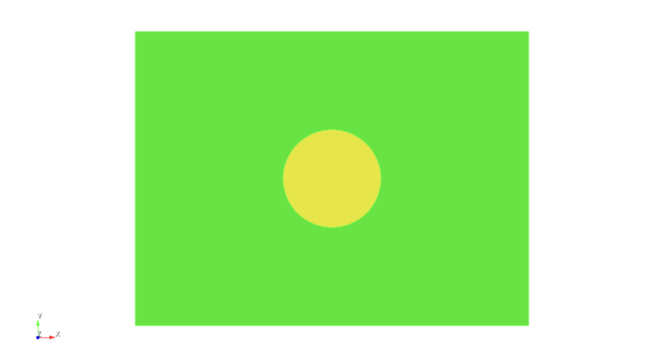
First, let's start by creating a rectangle and a circle. In Coreform Cubit, this can be
achieved using:
create surface rectangle width 2 height 1.5 zplane create surface circle radius 0.25 zplane
Note that currently the circle and the rectangle are completely disjoint from
each other. In order to remove this overlap between these two entities, the
boolean operator can be used to subtract the circle from the rectangle:
subtract surface 2 from surface 1 keep_tool
While the rectangle now has a circular cutout in its center, the boundaries
between the yellow circle and the green rectangle are not shared. The merge
tool can be used to consolidate these curves into one:
merge curve 5 6
We will use the following material properties for this example:
| Entity | Physics | VP | VS | RHO |
|---|---|---|---|---|
| Circle | Acoustic | 1500 | N/A | 1000 |
| Rectangle | Elastic | 4500 | 3000 | 2000 |
As a general rule of thumb, using approximately 2.0 elements per wavelength
tends to yield minimal numerical dispersion for most applications. For this
example we'll assume that we're using a source with a maximum resolved
frequency of 30 kHz, meaning that we can compute the approximate element size
in each region as
and
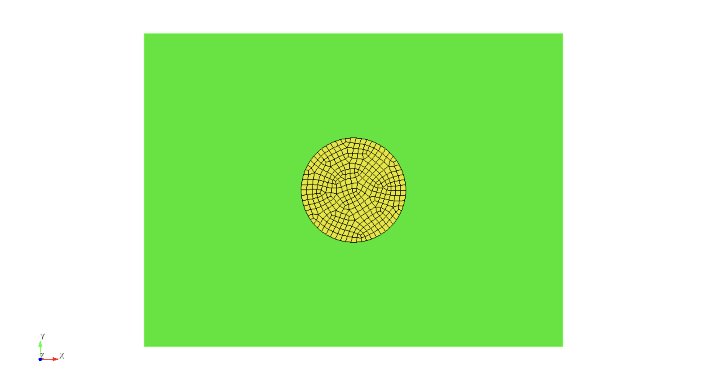
In order to mitigate spatial dispersion errors, it is advantageous to begin
meshing from the region with the finest discretization. Thus, first the
circular region is meshed with
surface 2 scheme pave
surface 2 size 0.025
mesh surface 2
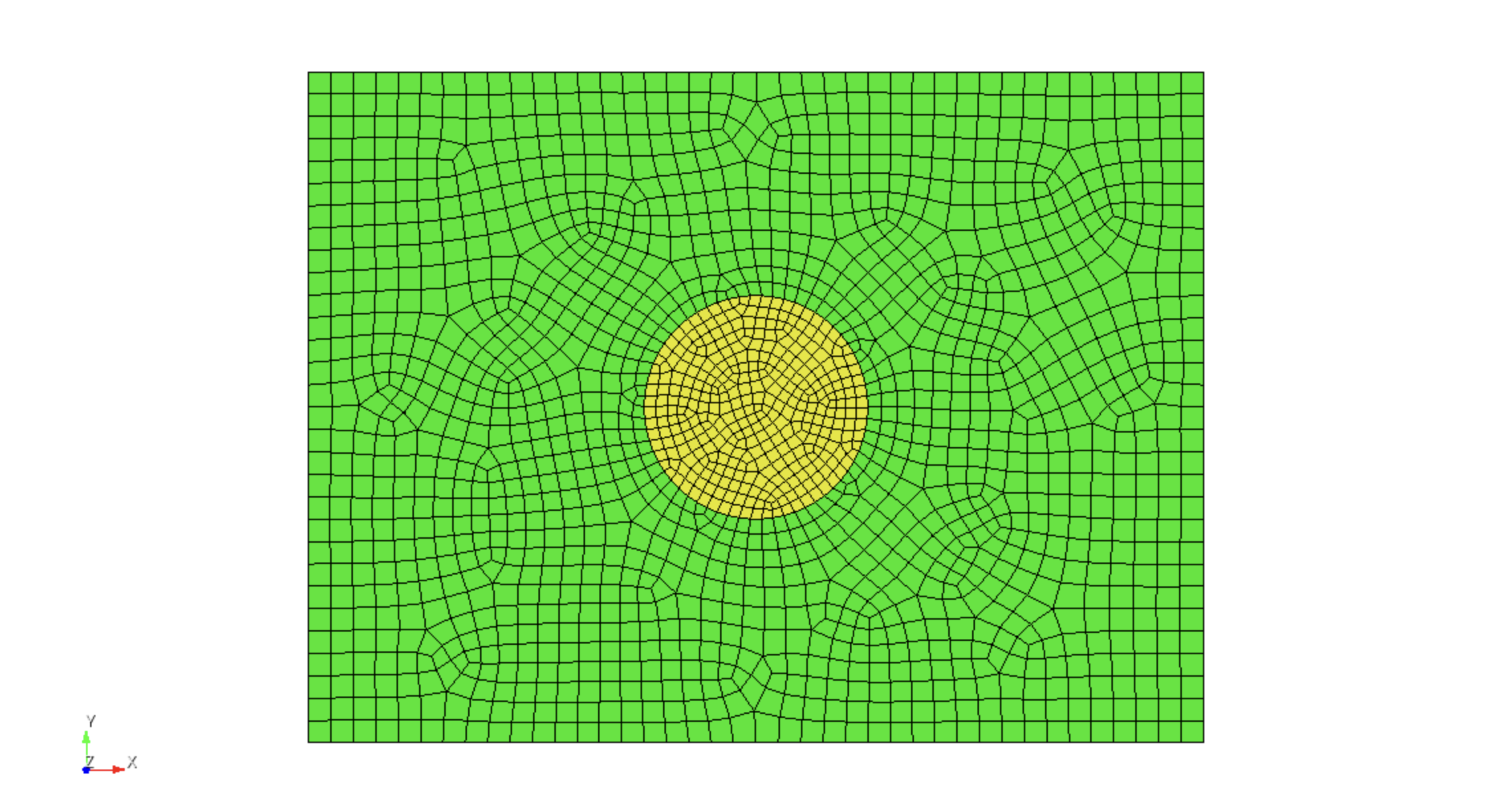
Next, the rectangular region is meshed using
surface 3 scheme pave
surface 3 size 0.05
surface 3 sizing function interval
mesh surface 3
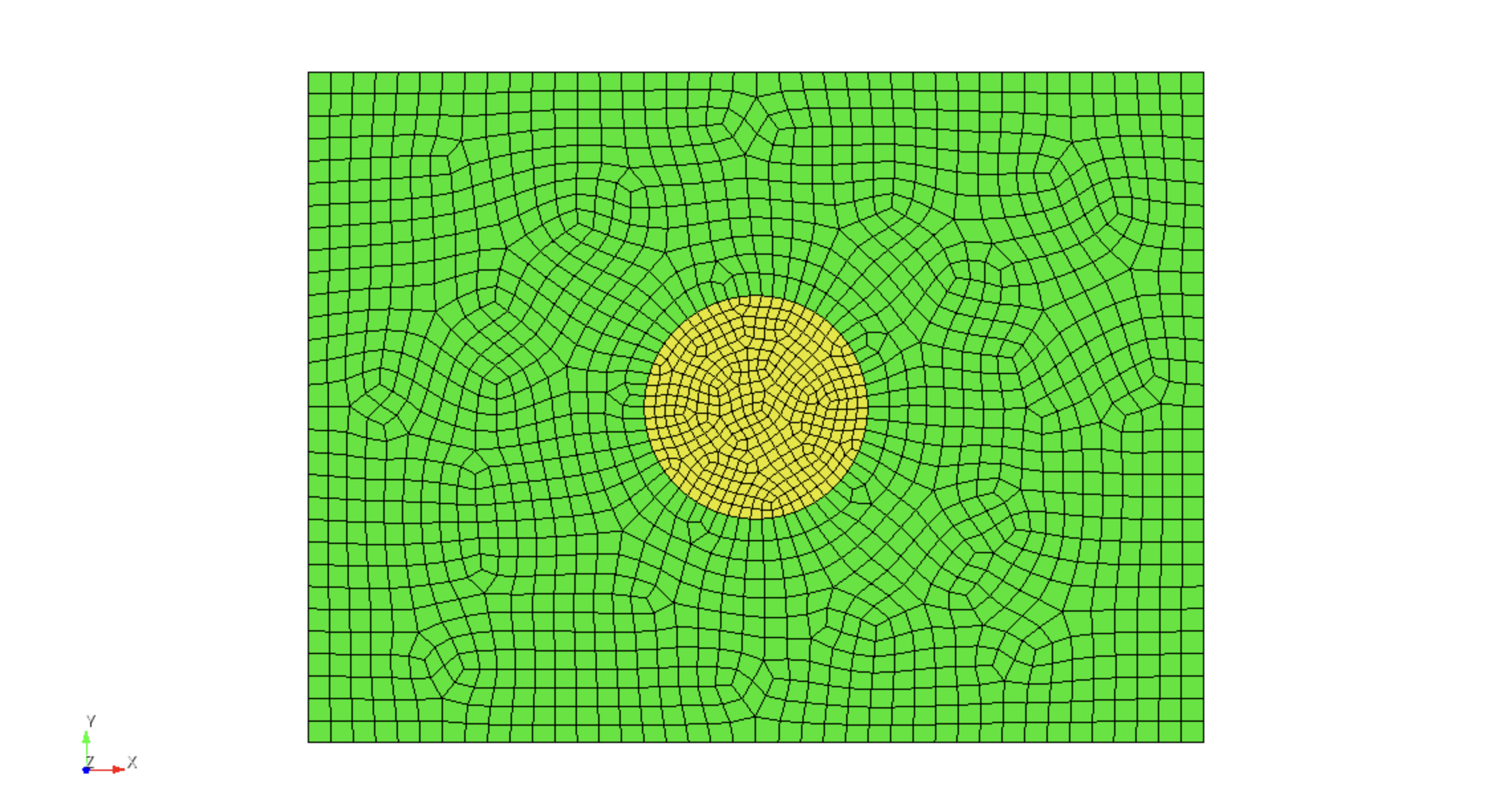
Mesh smoothing can be used to improve the uniformity of the element sizes
throughout the mesh using
surface all smooth scheme edge length
smooth surface all
In order to make it easier to select the individual discrete regions of the
mesh, we'll assign the circular inclusion as belonging to block 1, while the
surrounding part of the domain will belong to block 2:
block 1 add surface 2
block 2 add surface 3
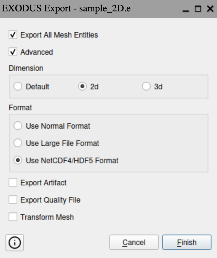
Finally, the mesh can be exported to Exodus such that it can be imported into
Salvus. It is important to export the mesh with the following settings:
- Dimensions: 2D
- Format: Use NetCDF4/HDF5 Format
This can be achieved using the Journal commands
set exodus netcdf4 on
export mesh "/path/to/file/sample_2D.e" dimension 2
Here's a complete list of the journal commands necessary for creating the mesh:
# Create the background rectangle and circular inclusion
create surface rectangle width 2 height 1.5 zplane
create surface circle radius 0.25 zplane

# Subtract the circle from the rectangle
subtract surface 2 from surface 1 keep_tool

# Merge overlapping curves
merge curve 5 6

# Mesh the circular region
surface 2 scheme pave
surface 2 size 0.025
mesh surface 2

# Mesh the rectangular region
surface 3 scheme pave
surface 3 size 0.05
surface 3 sizing function interval
mesh surface 3

# Smooth the mesh
surface all smooth scheme edge length
smooth surface all

# Assign the individual surfaces to blocks 1 and 2
block 1 add surface 2
block 2 add surface 3

# Export to Exodus
set exodus netcdf4 on
export mesh "/path/to/file/sample_2D.e" dimension 2
As usual, we'll start off by importing a few useful modules.
import os

import matplotlib.pyplot as plt
import numpy as np

from salvus.mesh.algorithms.unstructured_mesh.metrics import compute_time_step
import salvus.namespace as sn

SALVUS_FLOW_SITE_NAME = os.environ.get("SITE_NAME", "local")
RANKS_PER_JOB = 1
Let's begin by first importing the Exodus mesh. We can do this using the
from_exodus constructor that is part of the UnstructuredMesh class.
Here's an example of how we can do that:# Import the mesh; attach the block indices so that we can easily attach
# material properties afterwards
m_2d = sn.UnstructuredMesh.from_exodus(
"data/sample_2D.e", attach_element_block_indices=True
)
m_2d
<unstructured_mesh.unstructured_mesh.UnstructuredMesh object at 0x73fe47cf8e90>
Currently the mesh only has the block indices attached; we haven't specified
any other material properties yet. The block indices let us flag parts of
the mesh as belonging together and serve as a convenient way for
distinguishing between different discrete regions of the domain.
We can check for potential issues with the mesh using the
qc_test method:m_2d.qc_test()[2026-06-22 09:10:21,632] WARNING - salvus._core.validation: [INFO] 1 issues found: [critical] (mesh:NO_ELEMENT_NODAL_FIELDS) Mesh has no element nodal fields defined. Can't continue material quality control. Mitigation: Ensure the mesh has at least one element nodal field defined. ------------------------------------------------------------
{'mesh:NO_ELEMENT_NODAL_FIELDS': QCIssue(type='mesh', code='NO_ELEMENT_NODAL_FIELDS', message="Mesh has no element nodal fields defined. Can't continue material quality control.", severity=<QCIssueSeverity.critical: 50>, mitigation='Ensure the mesh has at least one element nodal field defined.', data={})}Uh oh — since we don't have any material properties attached yet, we wouldn't
be able to run a simulation just yet. Let's attach the material properties
that we defined earlier in the tutorial.
# Define our properties for the mesh
block_props = {
    1: {"VP": 1500.0, "RHO": 1000.0},
    2: {
        "VP": 4500.0,
        "VS": 3000.0,
        "RHO": 2000.0,
    },
}
We're going to want to assign all of the elements in each region of the mesh
to have these material properties. To do this, we can use the following
general recipe:
- Initialize each elemental field
- Create a mask that selects the elements for a particular block
- Assign the material properties from the
block_propsdictionary - Depending on whether the material is acoustic or elastic (i.e., whether
there is a
VSpresent), set thefluidflag for each region
def assign_properties_to_mesh(
    mesh: sn.UnstructuredMesh, properties: dict
) -> None:
    # Initialize the fluid flag
    mesh.attach_field("fluid", np.zeros(mesh.nelem, dtype=bool))

    # Initialize the elemental fields for the mesh
    for field in ["VP", "VS", "RHO"]:
        mesh.attach_field(field, np.zeros_like(mesh.connectivity, dtype=float))

    for block_id in properties:
        # Get the elements that belong to the given block ID
        mask = mesh.elemental_fields["element_block_index"] == block_id

        # Assign the material properties for that block
        for field, value in properties[block_id].items():
            mesh.elemental_fields[field][mask, :] = value

        # Set the fluid flag for the given block; this will tell the solver
        # whether to use the acoustic or elastic solver for that part of the
        # mesh
        if "VS" not in properties[block_id]:
            mesh.elemental_fields["fluid"][mask] = True
        else:
mesh.elemental_fields["fluid"][mask] = False# Assign the properties and visualize the mesh
assign_properties_to_mesh(m_2d, block_props)
m_2d
<unstructured_mesh.unstructured_mesh.UnstructuredMesh object at 0x73fe47cf8e90>
Let's run the
qc_test again to see if there are any remaining issues with
the mesh.m_2d.qc_test()[2026-06-22 09:10:21,863] INFO: [SUCCESS] No issues found!
{}It looks like we're good to go!
We checked before whether we'll be able to execute the simulation with the
mesh we've imported. While the
qc_test tells us if there are issues with
the mesh that will prevent us from running the simulation, it is still up to
the user to make sure that the external mesh has been constructed in such a
way that it will perform well for the simulation:- Having elements that are too large will introduce numerical dispersion errors into the simulation
- Having elements that are too small will limit the global time step under the Courant (or CFL) criterion, which will make the simulation much more computationally expensive to run.
To make sure that our simulation will perform well, there are two things we
want to check here:
- Compute the resolved frequencies of each element in the mesh to make sure that they're (mostly) around the desired maximum frequency of the source.
- Compute the time step to see where the limiting elements in the mesh are.
# Initialize an array that we'll use to track the minimum velocities in the
# mesh
min_velocity = np.zeros(m_2d.nelem, dtype=float)

for block_id, props in block_props.items():
    # Get the mask for the specific block
    mask = m_2d.elemental_fields["element_block_index"] == block_id

    # If the material property is elastic, use `VS`; otherwise use `VP`.  This
    # is because `VS` is always smaller than `VP`
    if "VS" in props:
        min_velocity[mask] = np.min(
            m_2d.elemental_fields["VS"][mask, :], axis=1
        )
    else:
        min_velocity[mask] = np.min(
            m_2d.elemental_fields["VP"][mask, :], axis=1
        )

# Calculate the resolved frequencies
min_frequency_2d, resolved_frequencies_2d = m_2d.estimate_resolved_frequency(
    min_velocity=min_velocity,
    elements_per_wavelength=2.0,
)

print("Minimum resolved frequency is %.2f kHz" % (min_frequency_2d / 1e3))

m_2d.attach_field("resolved_frequency", resolved_frequencies_2d)
Minimum resolved frequency is 23.06 kHz
# Change plotted field to `resolved_frequency`
m_2d
<unstructured_mesh.unstructured_mesh.UnstructuredMesh object at 0x73fe47cf8e90>
In the above plot, we can see that the range of resolved frequencies seems to
mostly be in the same range. Let's visualize these mesh statistics with a
histogram to see the frequencies that most of the elements are resolving:
def colored_histogram(
    data: np.ndarray,
    n_bins: int = 50,
    colormap: str = "coolwarm",
) -> None:
    counts, bins = np.histogram(data, bins=n_bins)

    fig = plt.figure(figsize=[10, 3])
    cmap = plt.get_cmap(colormap)
    colors = cmap(np.linspace(0, 1, len(bins) - 1))

    for i in range(len(bins) - 1):
        plt.bar(
            bins[i],
            counts[i],
            width=bins[i + 1] - bins[i],
            color=colors[i],
            edgecolor="black",
        )

    return fig, counts, bins


def plot_resolved_frequencies(
    resolved_frequencies: np.ndarray,
    n_bins: int = 50,
    colormap: str = "coolwarm",
) -> None:
    _, counts, bins = colored_histogram(
        resolved_frequencies / 1e3, n_bins, colormap
    )

    plt.annotate(
        "Elements\nToo Large",
        xy=(bins[0], max(counts) * 0.45),
        xytext=(bins[6], max(counts) * 0.45),
        arrowprops=dict(facecolor="black", arrowstyle="-|>", lw=1.5),
        ha="center",
        va="center",
    )
    plt.annotate(
        "Elements\nToo Small",
        xy=(bins[-1], max(counts) * 0.45),
        xytext=(bins[-7], max(counts) * 0.45),
        arrowprops=dict(facecolor="black", arrowstyle="-|>", lw=1.5),
        ha="center",
        va="center",
    )

    plt.title("Resolved Frequencies")
    plt.xlabel("Frequency [kHz]")
    plt.ylabel("Number of Elements")
    plt.show()


def plot_dt(
    dts: np.ndarray, n_bins: int = 50, colormap: str = "coolwarm_r"
) -> None:
    _, counts, bins = colored_histogram(dts, n_bins, colormap)

    plt.annotate(
        "Restricting\nTime Step",
        xy=(bins[0], max(counts) * 0.05),
        xytext=(bins[0], max(counts) * 0.3),
        arrowprops=dict(facecolor="black", arrowstyle="-|>", lw=1.5),
        ha="center",
        va="center",
    )

    plt.title("Time Steps")
    plt.xlabel(r"$\Delta t$ [$\mu$s]")
    plt.ylabel("Number of Elements")
    plt.show()


plot_resolved_frequencies(resolved_frequencies_2d)
We can see here that most of our elements are resolving frequencies that are
around 30kHz, which is the approximate maximum frequencies that our source
will have.
While there are some elements that are somewhat too large, they are
sufficiently few in number that the additional dispersion introduced by them
for the sake of this example will likely be minimal. However, depending on
the application, one may wish to go back and remesh this domain to eliminate
these large elements.
As noted before, the abnormally small elements will limit the global time
step. We can nicely visualize this by creating a similar histogram of the
time steps for each element:
dt_2d, dts_2d = compute_time_step(
    mesh=m_2d,
    max_velocity=m_2d.elemental_fields["VP"].max(axis=1),
)

print(f"Global time step: {dt_2d * 1e6:.2f} us")

plot_dt(dts_2d * 1e6, colormap="coolwarm_r")
Global time step: 0.46 us

The spread of time steps is relatively narrow, meaning there is no singular
element that is significantly smaller than its surrounding elments. Thus,
while it may be possible to further optimize the time step for this mesh, it
is of satisfactory quality.
Finally, we can visualize the time steps of each element using the mesh
visualization widget:
m_2d.attach_field("dt", dts_2d)

# Change plotted field to `dt`
m_2d
<unstructured_mesh.unstructured_mesh.UnstructuredMesh object at 0x73fe47cf8e90>
To demonstrate that this mesh actually works in a forward simulation, let's
set up a very minimalistic project and output a wavefield for it.
# Initialize a new project
p_2d = sn.Project.from_mesh(
    path="project_2D",
    mesh=m_2d,
    load_if_exists=True,
)

# Add an event that has a source placed in the middle of the mesh
p_2d.add_to_project(
    sn.Event(
        event_name="event_2D",
        sources=sn.simple_config.source.cartesian.ScalarPoint2D(
            x=0.0,
            y=0.0,
            f=1.0,
        ),
    )
)

# Run the simulation for 500 us
wsc = sn.WaveformSimulationConfiguration(end_time_in_seconds=500.0e-6)

# Use a Ricker wavelet; the max frequency of a Ricker is roughly 2x its center
# frequency
stf = sn.simple_config.stf.Ricker(center_frequency=30e3 / 2)
stf.plot()
# Create a new simulation configuration
p_2d.add_to_project(
    sn.UnstructuredMeshSimulationConfiguration(
        name="forward_simulation_2D",
        unstructured_mesh=m_2d,
        event_configuration=sn.EventConfiguration(
            waveform_simulation_configuration=wsc,
            wavelet=stf,
        ),
    )
)
Before running the simulation, let's check that the setup looks OK:
p_2d.viz.nb.simulation_setup(
    simulation_configuration="forward_simulation_2D",
    events="event_2D",
)
<salvus.flow.simple_config.simulation.waveform.Waveform object at 0x73fe3f1dba90>
Looks like we're good to go!
Here we'll output a few wavefield snapshots for the simulation. In order to
easily compare the outputs for the acoustic and elastic parts, we'll output
the fields
displacement and gradient-of-phi. We can convert the
gradient-of-phi in the acoustic part to displacement using the conversion
ofwhere is the displacement wavefield,
is the mass density (i.e., the
RHO field in the acoustic part of the mesh),
and is the gradient-of-phi wavefield that
we output in the acoustic part of the mesh.p_2d.simulations.launch(
simulation_configuration="forward_simulation_2D",
events="event_2D",
site_name=SALVUS_FLOW_SITE_NAME,
ranks_per_job=RANKS_PER_JOB,
extra_output_configuration={
"volume_data": {
"sampling_interval_in_time_steps": 25,
"fields": ["displacement", "gradient-of-phi"],
},
},
)[2026-06-22 09:10:23,268] INFO: Submitting job ... Uploading 1 files... 🚀 Submitted job_2606220910366463_34c1bf6046@local
1
p_2d.simulations.query(
    simulation_configuration="forward_simulation_2D",
    events="event_2D",
    block=True,
)
True
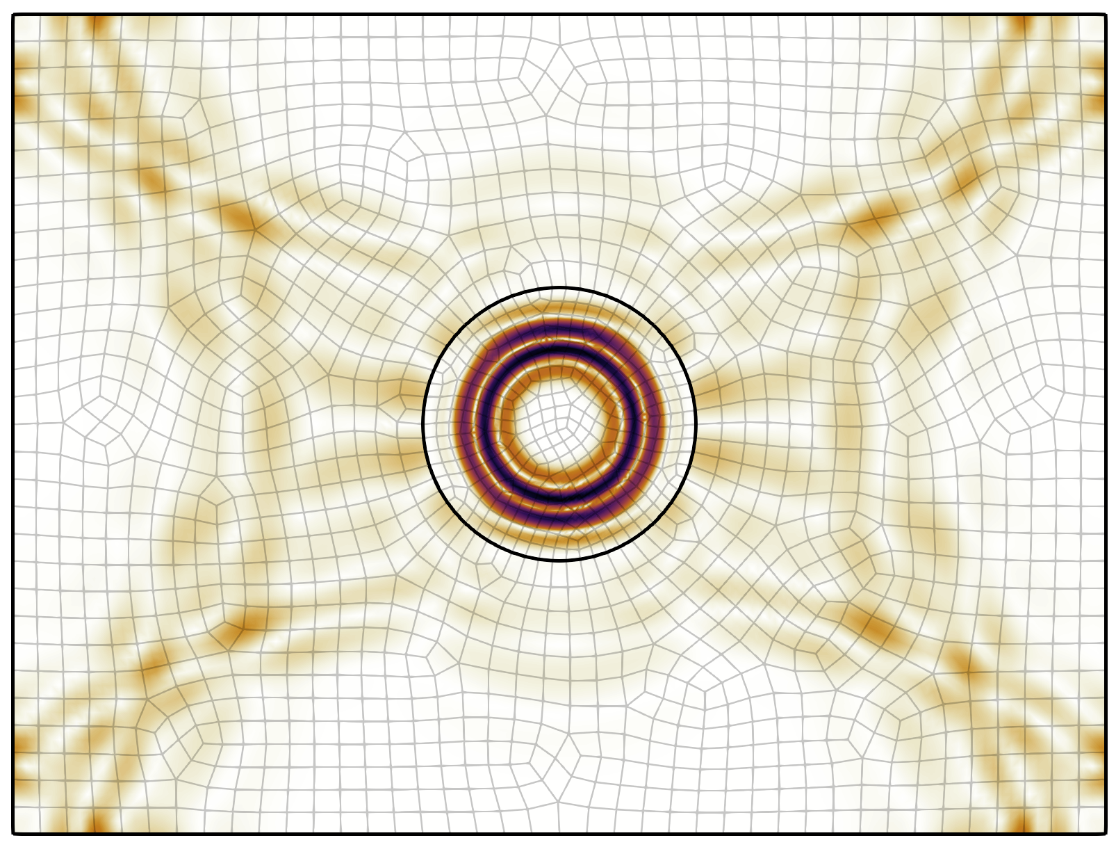
To visualize this data, one can use an application such as ParaView.
Included in this tutorial is a ParaView state file that can be used to load
in the necessary data for this. Here's a snapshot of what the wavefield
looks like at the final time step:

PAGE CONTENTS