As part of the W-Scan software suite, we offer a digital twin library that
includes a wide range of commercially available ultrasonic inspection
devices to easily simulate and image ultrasound NDT data. In this tutorial,
you will learn how to:
- Load a predefined instrument from the library.
- Plot the instrument and visualize its acquisition mode.
- Place an instrument onto a digitial twin of a specimen.
- Simulate ultrasound inspection data.
Let us start by importing the W-Scan instrument library and Salvus:
import matplotlib.pyplot as plt
import os

import salvus.namespace as sn
import wscan.instruments

SALVUS_FLOW_SITE_NAME = os.environ.get("SALVUS_FLOW_SITE_NAME", "local")We currently support a range of instruments from several of the large NDT
hardware manufacturers. If you are interested in simulating an instrument
that is currently missing from the library, please get in touch with us and
we will happily add the desired instrument.
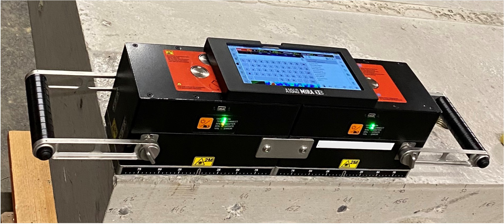
Let us now pick an instrument. For demonstration purposes, we use the ACS
Mira 3D Pro
device:
This instrument can record data in two different modes:
"matrix": This corresponds to the full matrix capture mode. Each transducer is fired separately and the data is recorded by each of the remaining transducers individually."linear": In linear mode, the transducers are fired row-wise, meaning that, for each shot, four transducers fire simultaneously. The data is then also recorded row-wise, meaning that the rows of 4 transducers are parallel-connected and their signal is combined into a single output channel.
The acquisition mode is defined upon loading the instrument. Here, we load
the instrument in both modes for demonstration purposes.
mira3d_pro_linear = wscan.instruments.get_instrument(
    instrument_name="acs-a1040-mira-3d-pro",
    acquisition_mode="linear",
)
mira3d_pro_matrix = wscan.instruments.get_instrument(
    instrument_name="acs-a1040-mira-3d-pro",
    acquisition_mode="matrix",
)
To better understand the recording sequence, it helps to visualize the
acquisition mode of the instrument in an interactive widget. You can
flip through the events by selecting them in the drop down menu on top. Each
event corresponds to one shot.
mira3d_pro_linear.plot_acquisition_mode()
Transducer elements marked with a red circle correspond to transducers that
act as a source for a given event (4 in linear mode). The receivers that are
parallel-connected are displayed in the same color. The numbers shown in the
receiving elements correspond to the index of this specific source-receiver
pair in the raw data output of this device. You can manually retrieve these
indices by calling the following:
receiver_ids = mira3d_pro_linear.receiver_ids
# 16 events in linear mode
assert len(receiver_ids) == 16

# IDs for the first event
receiver_ids[0]

# IDs for the last event. Note that in linear mode, the instrument records a
# total of 119 traces, as indicated by the last receiver id 119.
receiver_ids[-1]
[14, 28, 41, 53, 64, 74, 83, 91, 98, 104, 109, 113, 116, 118, 119]
Let us also visualize the
"matrix" mode, which results in data with 2016
traces.mira3d_pro_matrix.plot_acquisition_mode()
A detailed plot of the transducer layout and the instrument dimensions can be
obtained like this.
fig = plt.figure(figsize=(16, 4))
ax = plt.gca()
mira3d_pro_linear.plot(show_measurements=True, ax=ax)
In this tutorial, we will use the linear mode in order to avoid having to run
too many simulations.
We will use a pre-defined source time function from the
digital twin library that we can use for the simulations. This source time
function is derived from the specifications given to us by the instrument
manufacturer.
stf = mira3d_pro_linear.source_time_function.get_salvus_stf()
stf.plot()
If we have recorded data, we would typically use our auto-calibration
procedure to estimate the source time function directly from the data, as the
coupling of the device to the specimen might affect the source time function.
The automated calibration procedure is illustrated in a different tutorial.
If you want to limit the bandwidth of the source time function, you can
directly filter it like this:
stf_filtered = mira3d_pro_linear.source_time_function.bandpass_filter(
    min_frequency_in_hertz=40e3, max_frequency_in_hertz=60e3
).get_salvus_stf()
stf_filtered.plot()
Let us now set up a simulation. For this, we start by defining a domain.
Here, we use a simple 3D box domain mimicking a concrete slab with a length
of 1.0 meters, a width of 0.5 meters, and a height of 0.2 meters.
domain = sn.domain.dim3.BoxDomain(
    x0=0.0,
    x1=1.0,
    y0=0.0,
    y1=0.5,
    z0=-0.2,
    z1=0.0,
)
domain.plot()
We now set up a new Salvus project from this domain.
p = sn.Project.from_domain(
    domain=domain, path="project_acs", load_if_exists=True
)
We now want to place the instrument on the block. To do so, we will add an
orientation to it, which states where it is located and how it is oriented
(the instrument can be aribtrarily rotated in three dimensions). We specify
three properties:origin: The lower left corner of the instrument will be located at this point.normal_vector: This defines how the instrument is oriented in space.(0, 0, 1)specifies an upward pointing normal vector, meaning the transducers of the instrument lie in thexy-plane.rotation_angle_in_degrees: This will rotate the instrument by an aribtrary angle around the normal vector (counter-clockwise).
mira_on_block = mira3d_pro_linear.with_orientation(
    wscan.instruments.Orientation(
        origin=(
            0.1,
            0.1,
            0.0,
        ),  # x, y, and z coordinates of the lower right corner of the instrument
        normal_vector=(0, 0, 1),  # The normal vector of the instrument
        rotation_angle_in_degrees=0,  # The rotation of the instrument around the normal vector
    )
)
Let us again visualize the placed instrument on the block. Note that the
coordinates of the transducers now corresponds to their respective location on
the block.
mira_on_block.plot(zoom_to_fit=True)
We can now add the sources and receivers for this instrument location to our
project. To do so, we call the method
get_salvus_events, which should give
us 16 events in linear mode.events = mira_on_block.get_salvus_events(batch_identifier="dummy")
assert len(events) == 16
for event in events:
p.add_to_project(event)The events are now part of the project with names that enable us to identify
where the sources are fired.
p.events.list()['A1040 MIRA 3D PRO__batch_dummy__pos_000__shot_000__ori_x0.1000_y0.1000_z0.0000__nrm_x0.0000_y0.0000_z1.0000__rot_000__tx_mode_S-xline__acq_mode_linear', 'A1040 MIRA 3D PRO__batch_dummy__pos_000__shot_001__ori_x0.1000_y0.1000_z0.0000__nrm_x0.0000_y0.0000_z1.0000__rot_000__tx_mode_S-xline__acq_mode_linear', 'A1040 MIRA 3D PRO__batch_dummy__pos_000__shot_002__ori_x0.1000_y0.1000_z0.0000__nrm_x0.0000_y0.0000_z1.0000__rot_000__tx_mode_S-xline__acq_mode_linear', 'A1040 MIRA 3D PRO__batch_dummy__pos_000__shot_003__ori_x0.1000_y0.1000_z0.0000__nrm_x0.0000_y0.0000_z1.0000__rot_000__tx_mode_S-xline__acq_mode_linear', 'A1040 MIRA 3D PRO__batch_dummy__pos_000__shot_004__ori_x0.1000_y0.1000_z0.0000__nrm_x0.0000_y0.0000_z1.0000__rot_000__tx_mode_S-xline__acq_mode_linear', 'A1040 MIRA 3D PRO__batch_dummy__pos_000__shot_005__ori_x0.1000_y0.1000_z0.0000__nrm_x0.0000_y0.0000_z1.0000__rot_000__tx_mode_S-xline__acq_mode_linear', 'A1040 MIRA 3D PRO__batch_dummy__pos_000__shot_006__ori_x0.1000_y0.1000_z0.0000__nrm_x0.0000_y0.0000_z1.0000__rot_000__tx_mode_S-xline__acq_mode_linear', 'A1040 MIRA 3D PRO__batch_dummy__pos_000__shot_007__ori_x0.1000_y0.1000_z0.0000__nrm_x0.0000_y0.0000_z1.0000__rot_000__tx_mode_S-xline__acq_mode_linear', 'A1040 MIRA 3D PRO__batch_dummy__pos_000__shot_008__ori_x0.1000_y0.1000_z0.0000__nrm_x0.0000_y0.0000_z1.0000__rot_000__tx_mode_S-xline__acq_mode_linear', 'A1040 MIRA 3D PRO__batch_dummy__pos_000__shot_009__ori_x0.1000_y0.1000_z0.0000__nrm_x0.0000_y0.0000_z1.0000__rot_000__tx_mode_S-xline__acq_mode_linear', 'A1040 MIRA 3D PRO__batch_dummy__pos_000__shot_010__ori_x0.1000_y0.1000_z0.0000__nrm_x0.0000_y0.0000_z1.0000__rot_000__tx_mode_S-xline__acq_mode_linear', 'A1040 MIRA 3D PRO__batch_dummy__pos_000__shot_011__ori_x0.1000_y0.1000_z0.0000__nrm_x0.0000_y0.0000_z1.0000__rot_000__tx_mode_S-xline__acq_mode_linear', 'A1040 MIRA 3D PRO__batch_dummy__pos_000__shot_012__ori_x0.1000_y0.1000_z0.0000__nrm_x0.0000_y0.0000_z1.0000__rot_000__tx_mode_S-xline__acq_mode_linear', 'A1040 MIRA 3D PRO__batch_dummy__pos_000__shot_013__ori_x0.1000_y0.1000_z0.0000__nrm_x0.0000_y0.0000_z1.0000__rot_000__tx_mode_S-xline__acq_mode_linear', 'A1040 MIRA 3D PRO__batch_dummy__pos_000__shot_014__ori_x0.1000_y0.1000_z0.0000__nrm_x0.0000_y0.0000_z1.0000__rot_000__tx_mode_S-xline__acq_mode_linear', 'A1040 MIRA 3D PRO__batch_dummy__pos_000__shot_015__ori_x0.1000_y0.1000_z0.0000__nrm_x0.0000_y0.0000_z1.0000__rot_000__tx_mode_S-xline__acq_mode_linear']
For our simulations, we additionally need an
EventConfiguration stating the
simulation time and the source time function that we will use. We simply use
the default source time function of the Mira device that we have already seen
above.ec = sn.EventConfiguration(
wavelet=stf,
waveform_simulation_configuration=sn.WaveformSimulationConfiguration(
# We simulate 0.3 milliseconds of data
end_time_in_seconds=0.3e-3
),
)So far, we have not specified any material properties for our concrete slab;
let us do so now. To keep things simple, we will just simulate data for a
homogeneous block of concrete. Note that we have a data-driven calibration
procedure to automatically calibrate the velocities of our digital twin as
illustrated in a different tutorial. Here, we just use a fixed shear wave
velocity of 2800 m/s and a Vp/Vs ratio of 1.7.
# Define material properties of the concrete
concrete = sn.material.from_params(vp=1.7 * 2800, vs=2800.0, rho=2400.0)
Finally, we can set up our simulation and check if everything looks alright.
p += sn.SimulationConfiguration(
    name="simulation",
    elements_per_wavelength=1.25,
    # Simulation is accurate up to 70 kHz
    max_frequency_in_hertz=70_000,
    model_configuration=concrete,
    event_configuration=ec,
)

# Just show the first event of the firing sequence
p.viz.nb.simulation_setup("simulation", events=p.events.list()[0])
[2026-06-22 09:58:23,681] INFO: Creating mesh. Hang on.

<salvus.flow.simple_config.simulation.waveform.Waveform object at 0x7d7af39fc7d0>
This looks alright! So let's run the simulations. As you will see, we will
need to run 16 simulations to fully mimick the acquisition of the Mira Pro
device.
p.simulations.launch(
    simulation_configuration="simulation",
    events=p.events.list(),
    site_name=SALVUS_FLOW_SITE_NAME,
    ranks_per_job=4,
)
p.simulations.query(block=True)
[2026-06-22 09:58:24,142] INFO: Submitting job array with 16 jobs ...

True
Let's visualize the simulated data for two events using the Salvus waveform
retrieval.
ed_event_0 = p.waveforms.get("simulation", p.events.list()[0])[0]
# Get an xarray DataArray with the displacement data of this event
da = ed_event_0.get_waveform_data_xarray("displacement").unstack()
Note that Salvus will always simulate multicomponent data. The component
of interest for our instrument will always correspond to the first component
X, so we only need to extract that. Note that this is independent on the
orientation of the instrument. Salvus will always internally rotate the data
so that the first component corresponds to the instrument's main axis.
Let's plot this data.da.sel(component="X").plot()
plt.gca().set_ylim(0.0, 0.3e-3)(0.0, 0.0003)

Note that the data for this event contains 15 traces, each trace corresponds
to the combined output signal of four parallel-connected transducers of a
single row.
You can distinguish some distinct arrivals such as the direct wave, the
side-wall reflections, and the reflection from the bottom of the concrete
block.
Let us also look at an event from the middle of the firing sequence.
event_id = 6
ed_event_6 = p.waveforms.get("simulation", p.events.list()[event_id])[0]
# Get an xarray DataArray with the displacement data of this event
ed_event_6.get_waveform_data_xarray("displacement").unstack().sel(
    component="X"
).plot()
plt.gca().set_ylim(0.0, 0.3e-3)
(0.0, 0.0003)

Again, we can identify the direct wave, side-wall reflections, and the bottom
reflection and the data looks as expected for this simple configuration.
This concludes this first tutorial on simulating ultrasound inspection data
with the W-Scan instrument library. In future tutorials, we will illustrate
how to simulate more complex specimens with embedded defects, read actual
inspection data, and use the W-Scan library to process and image the data
using different ultrasound imaging algorithms.

PAGE CONTENTS